---
title: "Toy Models"
subtitle: "Understanding superposition in miniature"
author: "Taras Tsugrii"
date: 2025-01-05
categories: [core-theory, toy-models]
description: "Before tackling superposition in billion-parameter models, we study it in systems simple enough to fully understand. The insights transfer remarkably well."
---
::: {.callout-tip}
## What You'll Learn
- How to build the simplest possible network that exhibits superposition
- Why optimal arrangements form regular polytopes (pentagons, hexagons)
- How to observe and verify the phase transition experimentally
- Why Polya's "solve a simpler problem first" heuristic is essential
:::
::: {.callout-warning}
## Prerequisites
**Required**: [Chapter 6: Superposition](06-superposition.qmd) — understanding the superposition hypothesis and why sparsity matters
:::
::: {.callout-note}
## Before You Read: Recall
From Chapter 6, recall:
- Superposition: networks store more features than dimensions using *almost-orthogonal* directions
- Sparsity enables this: if features rarely co-occur, interference is manageable
- Phase transition: at critical sparsity, networks switch to superposition
- This is why polysemanticity exists and interpretation is hard
**Now we ask**: Can we study superposition in a controlled setting where we know the ground truth?
:::
## Solve a Simpler Problem First
In the previous chapter, we established that superposition is the central obstacle to mechanistic interpretability. Networks pack more features than dimensions, creating polysemantic neurons and hiding interpretable structure in a compressed representation.
But superposition in a real language model is hard to study. The model has billions of parameters, millions of features, and we don't know the ground truth—we don't know which features *should* exist or how they *should* be arranged.
This is where Polya's heuristic becomes essential: **solve a simpler problem first**.
What if we built a tiny network where:
- We know exactly how many features there are
- We control how sparse they are
- We can visualize the entire representation space
- We can verify whether the network finds the optimal arrangement
This is the toy model approach. Build a system simple enough to fully understand, observe superposition emerge, and use the insights to interpret real networks.
::: {.callout-note}
## The Core Idea
A toy model is an autoencoder trained to represent $n$ sparse features in $d < n$ dimensions. The network is forced to compress, and we can watch exactly how it chooses to do so.
:::
## The Setup
The Anthropic toy model has a beautifully simple architecture:
**Input**: A vector of $n$ features, where each feature is either "on" (value 1) or "off" (value 0). Each feature has a probability $S$ of being on—this is the sparsity parameter.
**Bottleneck**: A hidden layer with only $d$ dimensions, where $d < n$. This forces compression.
**Output**: A reconstruction of the original $n$-dimensional input.
**Training objective**: Minimize reconstruction error.
The setup looks like this:
```
Input (n dims)  →  Hidden (d dims)  →  Output (n dims)
    [n features]      [compressed]       [reconstructed]
```
For a concrete example: 5 features compressed into 2 dimensions. The network must somehow represent 5 things using only 2 numbers.
### Why This Forces Superposition
In 2 dimensions, you can have at most 2 orthogonal directions. If each feature got its own orthogonal direction, you could only represent 2 features perfectly.
But we're asking for 5 features. The network has a choice:
- Represent only the 2 most important features perfectly, ignore the other 3
- Represent all 5 imperfectly, accepting some interference
When features are sparse (rarely active), the second option is better. The network can pack 5 features into 2 dimensions as long as it accepts occasional errors when multiple features are active simultaneously.
This is superposition, and we can watch it emerge.
## The Pentagon Discovery
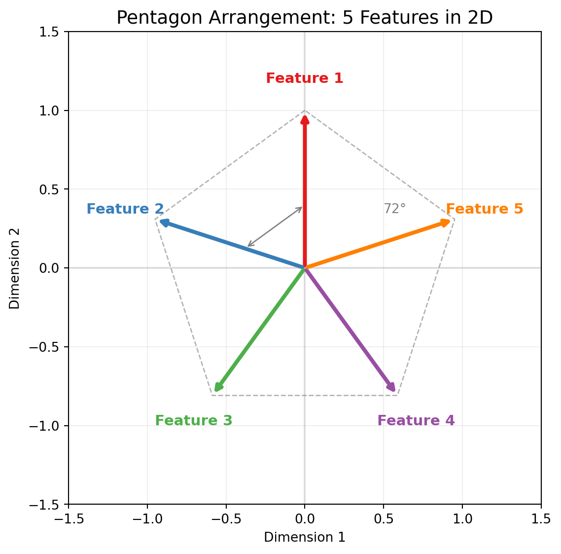
Here's what happens when you train this toy model with 5 sparse features in 2 dimensions:
The network learns to represent the 5 features as 5 directions arranged in a **regular pentagon**.
```
                F1
                ↑
               /|\
              / | \
          F5 ←--●--→ F2
              \ | /
               \|/
             ↙   ↘
           F4     F3
```
Each feature gets a direction. Adjacent features are 72° apart (360° / 5). No two features are orthogonal, but they're spread as far apart as possible.
::: {.callout-important}
## Why a Pentagon?
The pentagon arrangement minimizes the maximum interference between any two features. Any other arrangement would have some pair of features closer together, causing more interference when both are active. Gradient descent discovers this optimal geometry automatically.
:::
### Measuring the Geometry
We can verify the pentagon arrangement directly:
1. Extract the weight matrix $W$ that maps inputs to the hidden layer
2. Each column of $W$ is the direction for one feature
3. Compute the angle between each pair of feature directions
4. Observe that adjacent features are 72° apart, opposite features are 144° apart
The network has found the mathematically optimal arrangement without being told what it is. This is gradient descent discovering geometry.
```{python}
#| label: fig-pentagon
#| fig-cap: "5 features arranged as a pentagon in 2D. Adjacent features are 72° apart—the optimal arrangement that minimizes interference."
#| code-fold: true
import numpy as np
import matplotlib.pyplot as plt

fig, ax = plt.subplots(figsize=(6, 6))

# 5 features as a pentagon (72° spacing)
n_features = 5
angles = np.linspace(np.pi/2, np.pi/2 + 2*np.pi, n_features + 1)[:-1]  # Start from top

colors = ['#e41a1c', '#377eb8', '#4daf4a', '#984ea3', '#ff7f00']

for i, angle in enumerate(angles):
    # Draw arrow
    ax.annotate('', xy=(np.cos(angle), np.sin(angle)), xytext=(0, 0),
                arrowprops=dict(arrowstyle='->', color=colors[i], lw=3))
    # Label
    ax.text(1.2*np.cos(angle), 1.2*np.sin(angle), f'Feature {i+1}',
            ha='center', va='center', fontsize=11, fontweight='bold', color=colors[i])

# Draw the pentagon outline
pentagon_x = [np.cos(a) for a in angles] + [np.cos(angles[0])]
pentagon_y = [np.sin(a) for a in angles] + [np.sin(angles[0])]
ax.plot(pentagon_x, pentagon_y, 'k--', alpha=0.3, lw=1)

# Angle annotation
ax.annotate('', xy=(0.4*np.cos(angles[0]), 0.4*np.sin(angles[0])),
            xytext=(0.4*np.cos(angles[1]), 0.4*np.sin(angles[1])),
            arrowprops=dict(arrowstyle='<->', color='gray', lw=1))
ax.text(0.5, 0.35, '72°', fontsize=10, color='gray')

ax.set_xlim(-1.5, 1.5)
ax.set_ylim(-1.5, 1.5)
ax.set_aspect('equal')
ax.axhline(y=0, color='gray', linestyle='-', alpha=0.2)
ax.axvline(x=0, color='gray', linestyle='-', alpha=0.2)
ax.set_title('Pentagon Arrangement: 5 Features in 2D', fontsize=14)
ax.set_xlabel('Dimension 1')
ax.set_ylabel('Dimension 2')
ax.grid(True, alpha=0.2)

plt.tight_layout()
plt.show()
```
### Interactive: Explore Polytope Arrangements
Use the slider below to see how different numbers of features arrange themselves in 2D. Notice how the angles between features change as you add more.
```{ojs}
//| echo: false
viewof numFeatures = Inputs.range([3, 12], {step: 1, value: 5, label: "Number of features"})
```
```{ojs}
//| echo: false
{
  const width = 400;
  const height = 400;
  const radius = 150;
  const centerX = width / 2;
  const centerY = height / 2;

  // Calculate feature positions
  const features = [];
  for (let i = 0; i < numFeatures; i++) {
    const angle = (Math.PI / 2) + (2 * Math.PI * i / numFeatures);
    features.push({
      x: centerX + radius * Math.cos(angle),
      y: centerY - radius * Math.sin(angle),
      angle: angle,
      index: i + 1
    });
  }

  // Calculate angle between adjacent features
  const angleDegrees = (360 / numFeatures).toFixed(1);
  const cosineSimAdj = Math.cos(2 * Math.PI / numFeatures).toFixed(3);

  // Colors for features
  const colors = ["#e41a1c", "#377eb8", "#4daf4a", "#984ea3", "#ff7f00",
                  "#f781bf", "#a65628", "#999999", "#66c2a5", "#fc8d62",
                  "#8da0cb", "#e78ac3"];

  const svg = d3.create("svg")
    .attr("width", width)
    .attr("height", height)
    .attr("viewBox", [0, 0, width, height]);

  // Draw axes
  svg.append("line")
    .attr("x1", 20).attr("y1", centerY)
    .attr("x2", width - 20).attr("y2", centerY)
    .attr("stroke", "#ccc").attr("stroke-width", 1);
  svg.append("line")
    .attr("x1", centerX).attr("y1", 20)
    .attr("x2", centerX).attr("y2", height - 20)
    .attr("stroke", "#ccc").attr("stroke-width", 1);

  // Draw polygon outline
  const polygonPoints = features.map(f => `${f.x},${f.y}`).join(" ");
  svg.append("polygon")
    .attr("points", polygonPoints)
    .attr("fill", "none")
    .attr("stroke", "#333")
    .attr("stroke-width", 1)
    .attr("stroke-dasharray", "4,2")
    .attr("opacity", 0.3);

  // Draw feature vectors
  features.forEach((f, i) => {
    // Arrow line
    svg.append("line")
      .attr("x1", centerX).attr("y1", centerY)
      .attr("x2", f.x).attr("y2", f.y)
      .attr("stroke", colors[i % colors.length])
      .attr("stroke-width", 3);

    // Arrowhead
    const arrowSize = 10;
    const angle = Math.atan2(centerY - f.y, f.x - centerX);
    svg.append("polygon")
      .attr("points", `${f.x},${f.y} ${f.x - arrowSize * Math.cos(angle - 0.3)},${f.y + arrowSize * Math.sin(angle - 0.3)} ${f.x - arrowSize * Math.cos(angle + 0.3)},${f.y + arrowSize * Math.sin(angle + 0.3)}`)
      .attr("fill", colors[i % colors.length]);

    // Label
    const labelRadius = radius + 25;
    svg.append("text")
      .attr("x", centerX + labelRadius * Math.cos(f.angle))
      .attr("y", centerY - labelRadius * Math.sin(f.angle))
      .attr("text-anchor", "middle")
      .attr("dominant-baseline", "middle")
      .attr("font-size", "12px")
      .attr("font-weight", "bold")
      .attr("fill", colors[i % colors.length])
      .text(`F${f.index}`);
  });

  // Info text
  svg.append("text")
    .attr("x", centerX).attr("y", height - 40)
    .attr("text-anchor", "middle")
    .attr("font-size", "14px")
    .text(`${numFeatures} features → ${angleDegrees}° between adjacent`);

  svg.append("text")
    .attr("x", centerX).attr("y", height - 20)
    .attr("text-anchor", "middle")
    .attr("font-size", "12px")
    .attr("fill", "#666")
    .text(`Adjacent cosine similarity: ${cosineSimAdj}`);

  return svg.node();
}
```
::: {.callout-note}
## What to Notice
- As you add more features, the angle between adjacent features shrinks
- More features → higher cosine similarity → more interference when multiple are active
- At some point (depending on sparsity), adding more features isn't worth the interference cost
- This is why the phase transition exists: there's a limit to useful superposition
:::
## Phase Transitions
The most striking finding from toy model experiments is the **phase transition**.
As you vary the sparsity parameter $S$ (how often features are active), the network's behavior changes *discontinuously*.
### High Sparsity (Rare Features)
When $S$ is small (say, 0.01—each feature active 1% of the time):
- Features almost never co-occur
- Interference is rare and worth accepting
- Network uses heavy superposition
- All 5 features get directions, arranged as a pentagon
- Reconstruction quality is high except in rare cases
### Low Sparsity (Common Features)
When $S$ is large (say, 0.3—each feature active 30% of the time):
- Features frequently co-occur
- Interference happens constantly
- Superposition is too costly
- Network dedicates dimensions to the most important features
- Less important features are ignored entirely
### The Transition
Between these regimes, there's a **sharp threshold**. At some critical sparsity $S^*$, the network's strategy flips:
- Below $S^*$: superposed representation (pentagon)
- Above $S^*$: dedicated representation (subset of features)
The transition isn't gradual. Small changes in sparsity near the threshold cause the network to completely reorganize its representation.
```{python}
#| label: fig-phase-transition
#| fig-cap: "Phase transition in superposition: as sparsity decreases (features become more common), the network suddenly switches from superposed representation to dedicated representation."
#| code-fold: true
import numpy as np
import matplotlib.pyplot as plt

fig, (ax1, ax2) = plt.subplots(1, 2, figsize=(11, 4))

# Simulated phase transition curve
sparsity = np.linspace(0.01, 0.5, 100)
# Sigmoid-like sharp transition around S* = 0.15
features_represented = 5 / (1 + np.exp(25 * (sparsity - 0.15))) + 2 * (1 - 1/(1 + np.exp(25 * (sparsity - 0.15))))

ax1.plot(sparsity, features_represented, 'b-', lw=2.5)
ax1.axvline(x=0.15, color='red', linestyle='--', alpha=0.7, label='Critical sparsity S*')
ax1.fill_between(sparsity[sparsity < 0.15], 0, 5.5, alpha=0.1, color='green')
ax1.fill_between(sparsity[sparsity >= 0.15], 0, 5.5, alpha=0.1, color='orange')
ax1.text(0.07, 4.8, 'Superposition\n(all 5 features)', fontsize=9, ha='center', color='green')
ax1.text(0.32, 2.5, 'Dedicated\n(2 features)', fontsize=9, ha='center', color='orange')
ax1.set_xlabel('Feature Activation Probability (S)', fontsize=11)
ax1.set_ylabel('Features Represented', fontsize=11)
ax1.set_title('Phase Transition: Features vs Sparsity', fontsize=12)
ax1.set_ylim(0, 5.5)
ax1.set_xlim(0, 0.5)
ax1.legend(loc='upper right')
ax1.grid(True, alpha=0.3)

# Reconstruction loss
loss_superposed = 0.02 + 0.5 * sparsity**2  # Low base + interference at high density
loss_dedicated = 0.15 * np.ones_like(sparsity)  # Constant (3/5 features missing)
optimal_loss = np.minimum(loss_superposed, loss_dedicated)

ax2.plot(sparsity, loss_superposed, 'g--', lw=2, label='Superposition strategy', alpha=0.7)
ax2.plot(sparsity, loss_dedicated, 'orange', linestyle='--', lw=2, label='Dedicated strategy', alpha=0.7)
ax2.plot(sparsity, optimal_loss, 'b-', lw=2.5, label='Optimal (network chooses)')
ax2.axvline(x=0.15, color='red', linestyle='--', alpha=0.7)
ax2.set_xlabel('Feature Activation Probability (S)', fontsize=11)
ax2.set_ylabel('Reconstruction Loss', fontsize=11)
ax2.set_title('Why the Transition Happens', fontsize=12)
ax2.set_xlim(0, 0.5)
ax2.legend(loc='upper left', fontsize=9)
ax2.grid(True, alpha=0.3)

plt.tight_layout()
plt.show()
```
::: {.callout-tip}
## A Physical Analogy
Phase transitions in toy models are like phase transitions in physics—water freezing, or magnets aligning. The system doesn't gradually shift; it snaps from one qualitative state to another. The underlying mathematics is similar: optimization landscapes with multiple local minima, and sudden switches between them.
:::
## Polytope Arrangements
The pentagon is just one example. The general pattern: networks arrange features as vertices of **regular polytopes**—the higher-dimensional generalizations of regular polygons.
### Examples
**4 features in 2D**: Square (90° between adjacent features)
**6 features in 2D**: Hexagon (60° between adjacent features)
**4 features in 3D**: Tetrahedron (109.5° between all pairs)
**6 features in 3D**: Octahedron
The pattern is consistent: maximize the minimum angle between any two features. This minimizes worst-case interference.
### Why Polytopes?
The loss function penalizes reconstruction error. When features interfere (because they're not orthogonal), reconstruction suffers. The network minimizes total interference by spreading features as far apart as possible.
For $k$ features in $d$ dimensions where $k > d$, the optimal arrangement is the vertices of a regular polytope with $k$ vertices. This is a known result in geometric optimization, and neural networks rediscover it through gradient descent.
::: {.callout-note}
## Emergent Optimality
No one programs these arrangements. The network simply tries to minimize reconstruction error, and the geometry falls out. This suggests that optimization pressure is enough to find elegant mathematical solutions—a recurring theme in deep learning.
:::
## The Mathematics
Let's be more precise about interference and why polytopes are optimal.
### Interference Cost
When two features have directions $\mathbf{w}_1$ and $\mathbf{w}_2$ with cosine similarity $c = \mathbf{w}_1 \cdot \mathbf{w}_2$, the interference when both are active is proportional to $c$.
If feature 1 is active and feature 2 should be inactive, but they share direction, the reconstruction will incorrectly activate feature 2 by amount $\approx c$.
The expected interference cost depends on:
- How often features co-occur ($\propto S^2$ if independent)
- How aligned their directions are ($\propto c^2$ for squared error)
### The Trade-off
The network optimizes:
$$\text{Total Loss} = \text{Capacity Loss} + \text{Interference Loss}$$
- **Capacity Loss**: Features that don't get represented at all contribute to error whenever they're active
- **Interference Loss**: Superposed features contribute error when they co-occur
At high sparsity, interference loss is low (features rarely co-occur), so the network superimposes aggressively to minimize capacity loss.
At low sparsity, interference loss dominates, so the network reserves dimensions for important features and ignores others.
### Optimal Angles
For $k$ features superposed in $d$ dimensions, the optimal arrangement has:
- All features equidistant from each other (in angle)
- Minimum pairwise cosine similarity
For the pentagon in 2D: $\cos(72°) \approx 0.31$. For the hexagon: $\cos(60°) = 0.5$.
More features means smaller angles, which means more interference. Eventually, the interference cost exceeds the benefit, and it's better to drop features than to pack more.
## Visualizing Superposition
One of the great virtues of toy models is that we can *see* what's happening.
### Weight Matrix Visualization
The weight matrix $W$ maps features to hidden dimensions. Each column of $W$ is a feature's direction in the hidden space.
For 5 features in 2D, $W$ is a 2×5 matrix. Plotting the 5 columns as vectors in 2D directly shows the pentagon arrangement.
### Activation Patterns
When a specific input (say, features 1 and 3 both active) passes through the network:
1. The hidden activation is the sum of feature 1's direction and feature 3's direction
2. The reconstruction projects this back to all 5 features
3. Features 1 and 3 reconstruct strongly; others reconstruct weakly (but not zero—this is interference)
You can visualize which hidden dimensions "light up" for which features, and see the polysemanticity directly: each hidden dimension participates in multiple features.
### Training Dynamics
Watching training in real-time reveals how the network discovers the optimal geometry:
1. Initially, feature directions are random
2. Gradient descent pushes features apart (to reduce interference)
3. Features rotate toward the polytope arrangement
4. The arrangement stabilizes when each feature is equidistant from its neighbors
The optimization process is a geometric dance, and toy models let us watch every step.
## What Transfers to Real Models
The toy model findings aren't just academic curiosities. They predict real phenomena in large language models.
### Superposition Ratio
Anthropic's work on Claude 3 Sonnet found over 2 million interpretable features in a 4,096-dimensional layer. That's a ratio of ~500 features per dimension.
Toy models predict exactly this: when features are sparse enough (as they are in natural language), you can pack exponentially more features than dimensions.
### Sparsity Matches
Real features are sparse. The "Golden Gate Bridge" feature activates on ~0.05% of inputs. Most semantic features activate on less than 1% of inputs.
This matches the toy model regime where superposition is optimal—sparsity below ~1% enables heavy compression without unbearable interference.
### Polysemanticity Explained
The polysemantic neuron from Chapter 5 (cat faces + car fronts) is exactly what toy models predict. Each neuron participates in multiple feature directions. Looking at a single neuron shows a confusing mix; looking at the feature direction shows a clean concept.
### Steering Works
Adding a feature direction to activations shifts behavior predictably. This only works because features are linear directions—exactly the geometry that toy models reveal.
::: {.callout-tip}
## The Transfer Principle
Toy models operate by the same mathematical principles as large models: gradient descent finding efficient representations of sparse features in limited dimensions. The numbers differ (5 vs. 2 million features), but the geometry is the same.
:::
## What Doesn't Transfer
Toy models are deliberately simple. Some aspects don't generalize.
### Ground Truth
In toy models, we know the true features—we created them. In real models, we don't know which features the model "should" have. We're inferring features from behavior, not checking against ground truth.
### Feature Complexity
Toy model features are binary (on/off) and independent. Real features are continuous, context-dependent, and hierarchically organized. "French" doesn't just turn on and off; it has degrees and interacts with other concepts.
### Architecture
Toy models are simple autoencoders. Real transformers have attention, layer norms, residual connections, and dozens of layers. The compositional structure of transformers creates phenomena (like induction heads, which we'll cover in Chapter 13) that don't appear in toy models.
### Scale
5 features in 2 dimensions is tractable. 2 million features in 4,096 dimensions is a different beast. The principles may transfer, but the practical challenges of discovery and verification are much harder.
### Reconstruction Errors
When sparse autoencoders are trained on real model activations, they show 10-40% reconstruction error. This suggests the clean superposition picture from toy models is only approximate in practice. Real representations are messier.
::: {.callout-important}
## The Limitation
Toy models teach principles, not details. They explain *why* superposition exists and *how* it works geometrically. They don't tell us exactly which features a real model uses or how to find them efficiently.
:::
## Pedagogy: Why This Matters
Toy models aren't just research tools. They're essential for building intuition.
### Making the Abstract Concrete
"Features are directions in activation space" is abstract. Seeing a pentagon of 5 features in 2D makes it concrete. You can plot it, measure angles, verify predictions.
### Demystifying Optimization
"Gradient descent finds efficient representations" sounds magical. Watching a toy model rotate its weight vectors toward the optimal polytope demystifies it. Optimization is just following the gradient, and the gradient points toward good geometry.
### Building Transferable Intuition
Once you understand that 5 features form a pentagon in 2D, you have a mental model for what 2 million features might look like in 4,096D. You can't visualize it directly, but you understand the *kind* of structure that exists.
### Enabling Experimentation
Anyone can train a toy model in an afternoon. You can vary sparsity, count features, change dimensions, and observe results. This hands-on experimentation builds intuition that reading papers cannot.
## Polya's Perspective: The Simpler Problem
This chapter is a direct application of Polya's heuristic: **if you can't solve a problem, solve a simpler problem first**.
Superposition in GPT-4 is too complex to study directly. But superposition in a 5-feature, 2-dimensional autoencoder is fully tractable. We can:
- Verify that superposition occurs
- Observe the optimal geometry
- Measure the phase transitions
- Predict when superposition will vs. won't happen
Then we take these insights and apply them to the hard problem. We know what to look for. We know the geometry should be polytope-like. We know sparsity is the key parameter. We know polysemanticity is a cross-section of superposed directions.
::: {.callout-tip}
## Polya's Insight
"If you can't solve the problem, look for a related problem that you *can* solve." Toy models are that related problem. They share the essential structure (superposition) while removing the incidental complexity (billions of parameters, unknown features, compositional architecture).
:::
## Looking Ahead
We've now seen superposition in action—concrete, visual, fully understood.
But features in isolation don't explain how models *compute*. A language model doesn't just represent "French" and "cooking" as separate features; it combines them to process "French cuisine" and predict appropriate continuations.
How do features compose? How do multiple components work together to perform a computation? This is the question of **circuits**—the subject of the next chapter.
If features are atoms, circuits are molecules. And just as understanding atoms prepared chemists to understand molecules, understanding features prepares us to understand how they combine into computational structures.
---
## Further Reading
1. **Toy Models of Superposition** — [Anthropic](https://transformer-circuits.pub/2022/toy_model/index.html): The foundational paper. Essential reading with interactive visualizations.
2. **Interactive Toy Model** — [Mitchell Gordon](https://mitchgordon.me/ToyModels/): Train toy models in your browser and watch superposition emerge in real time.
3. **Toy Models of Superposition: A Walkthrough** — [Neel Nanda](https://www.neelnanda.io/mechanistic-interpretability/toy-model-walkthrough): Step-by-step guide to understanding and reproducing the experiments.
4. **The Persian Rug: Solving Toy Models Analytically** — [arXiv:2410.12101](https://arxiv.org/abs/2410.12101): Mathematical analysis proving optimality of polytope arrangements.
5. **Dynamical versus Bayesian Phase Transitions** — [arXiv:2310.06301](https://arxiv.org/abs/2310.06301): Deep dive into the phase transition phenomenon and its mathematical structure.
6. **Scaling Monosemanticity** — [Anthropic](https://transformer-circuits.pub/2024/scaling-monosemanticity/index.html): Applying toy model insights to real models, finding millions of features in Claude.