---
title: "Activations as Geometry"
subtitle: "Thinking in directions, not numbers"
author: "Taras Tsugrii"
date: 2025-01-05
categories: [foundations, geometry]
description: "The residual stream is a vector space. Understanding its geometry—what directions mean, how concepts are arranged, why high dimensions behave strangely—is the key to understanding what neural networks represent."
---
::: {.callout-tip}
## What You'll Learn
- Why activations should be thought of as points in high-dimensional space
- What "king - man + woman = queen" reveals about representations
- The linear representation hypothesis and why it enables interpretability
- Why high dimensions are both a curse (distance noise) and blessing (near-orthogonality)
:::
::: {.callout-warning}
## Prerequisites
**Required**: [Chapter 3: The Residual Stream](03-residual-stream.qmd) — understanding the shared workspace model
:::
::: {.callout-note}
## Before You Read: Recall
From Chapter 3, recall:
- What is the residual stream? (A shared vector that accumulates contributions from all components)
- How do components communicate? (By reading from and writing to the residual stream)
- What does the logit lens reveal? (Predictions refine progressively through layers)
:::
## A Famous Equation
In 2013, researchers at Google trained a neural network on billions of words and discovered something remarkable. The network learned to represent words as vectors—points in a 300-dimensional space. That much was expected.
What wasn't expected was the geometry.
**Now we ask**: The residual stream is a vector. But what *structure* does that vector have? What does it mean for concepts to be "directions"?
When researchers computed:
$$\text{king} - \text{man} + \text{woman}$$
they got a vector very close to **queen**.
This wasn't programmed. No one told the network that royalty minus masculinity plus femininity should equal a different royal title. The relationship emerged from training on raw text. The network had discovered that gender is a *direction* in its representational space, and that direction is consistent across different concepts.
::: {.callout-note}
## The Key Surprise
Vector arithmetic on learned representations produces semantically meaningful results. This suggests that meaning itself has geometric structure—that concepts aren't stored as arbitrary patterns, but as organized directions and regions in a high-dimensional space.
:::
This chapter is about that geometry. We've established that transformers are matrix multiplication machines (Chapter 2) and that information flows through a shared residual stream (Chapter 3). Now we ask: what's the *structure* of that stream? What does it mean for a concept to be a "direction"? And why does high-dimensional geometry enable representations far richer than we might expect?
The answers will set up everything that follows. Features ([Chapter 5](05-features.qmd)), superposition ([Chapter 6](06-superposition.qmd)), circuits ([Chapter 8](08-circuits.qmd))—all of these build on the geometric perspective we develop here.
## From Numbers to Geometry
Let's start with a shift in thinking.
The residual stream at any point in a transformer is a vector—say, 768 floating-point numbers. We could think of this as a list of values, each number meaning something. But this is the wrong frame.
Instead, think of the vector as a **point in 768-dimensional space**.
This isn't just a metaphor. It's mathematically precise:
- Each of the 768 dimensions is an axis
- The vector specifies a location along each axis
- The result is a single point in $\mathbb{R}^{768}$
We can't visualize 768 dimensions, but we can reason about them. The same geometric concepts that work in 2D and 3D—distance, direction, angle, projection—generalize cleanly to any number of dimensions.
And here's the crucial insight: **geometric relationships often carry semantic meaning**.
Two vectors that are close together (small Euclidean distance) tend to represent similar concepts. Two vectors pointing in similar directions (small angle between them) tend to share properties. The geometry isn't arbitrary; it reflects the structure of what the network has learned.
## Distance Has Meaning
Consider what happens when you embed similar words.
In a well-trained embedding space, "dog" and "puppy" are nearby—their vectors have small Euclidean distance. "Dog" and "democracy" are far apart. The network has learned that some tokens are more related than others, and this relationship manifests as spatial proximity.
This extends beyond single tokens. When a transformer processes the phrase "The capital of France is", the residual stream at the final position encodes the *context*, not just the last token. That encoded context is a point in space. Similar contexts—"The capital of Germany is", "France's capital city is"—produce nearby points. Unrelated contexts produce distant points.
We can measure this. Cosine similarity—the cosine of the angle between two vectors—is a standard way to quantify how "similar" two representations are:
$$\text{similarity}(a, b) = \frac{a \cdot b}{||a|| \cdot ||b||}$$
Values near 1 mean the vectors point in nearly the same direction. Values near 0 mean they're nearly perpendicular. Values near -1 mean they point in opposite directions.
### Interactive: Explore Cosine Similarity
Drag the sliders to change the angle of vector B and see how cosine similarity changes. Notice how similar directions have high similarity, perpendicular vectors have zero similarity, and opposite directions have negative similarity.
```{ojs}
//| label: fig-cosine-interactive
//| fig-cap: "Interactive cosine similarity: adjust vector B's angle to see how similarity changes with direction."
viewof angleB = Inputs.range([0, 360], {step: 1, value: 30, label: "Vector B angle (degrees)"})

// Vector A is fixed at 0 degrees
angleA = 0

// Calculate cosine similarity
cosineSim = Math.cos((angleB - angleA) * Math.PI / 180)
angleDiff = Math.abs(angleB - angleA) > 180 ? 360 - Math.abs(angleB - angleA) : Math.abs(angleB - angleA)

// Visualization
{
  const width = 450;
  const height = 350;
  const radius = 130;
  const cx = width / 2;
  const cy = height / 2 + 20;

  const svg = d3.create("svg")
    .attr("viewBox", [0, 0, width, height])
    .attr("width", width)
    .attr("height", height);

  // Background
  svg.append("circle")
    .attr("cx", cx).attr("cy", cy)
    .attr("r", radius)
    .attr("fill", "none")
    .attr("stroke", "#ddd")
    .attr("stroke-width", 1);

  // Axes
  svg.append("line").attr("x1", cx - radius).attr("y1", cy).attr("x2", cx + radius).attr("y2", cy).attr("stroke", "#eee");
  svg.append("line").attr("x1", cx).attr("y1", cy - radius).attr("x2", cx).attr("y2", cy + radius).attr("stroke", "#eee");

  // Vector A (fixed at 0 degrees - pointing right)
  const axA = Math.cos(angleA * Math.PI / 180) * radius * 0.9;
  const ayA = -Math.sin(angleA * Math.PI / 180) * radius * 0.9;
  svg.append("line")
    .attr("x1", cx).attr("y1", cy)
    .attr("x2", cx + axA).attr("y2", cy + ayA)
    .attr("stroke", "#e41a1c")
    .attr("stroke-width", 4);
  svg.append("circle").attr("cx", cx + axA).attr("cy", cy + ayA).attr("r", 6).attr("fill", "#e41a1c");
  svg.append("text").attr("x", cx + axA + 15).attr("y", cy + ayA + 5).attr("fill", "#e41a1c").attr("font-weight", "bold").text("A");

  // Vector B (adjustable)
  const axB = Math.cos(angleB * Math.PI / 180) * radius * 0.9;
  const ayB = -Math.sin(angleB * Math.PI / 180) * radius * 0.9;
  svg.append("line")
    .attr("x1", cx).attr("y1", cy)
    .attr("x2", cx + axB).attr("y2", cy + ayB)
    .attr("stroke", "#377eb8")
    .attr("stroke-width", 4);
  svg.append("circle").attr("cx", cx + axB).attr("cy", cy + ayB).attr("r", 6).attr("fill", "#377eb8");
  svg.append("text").attr("x", cx + axB + 15).attr("y", cy + ayB + 5).attr("fill", "#377eb8").attr("font-weight", "bold").text("B");

  // Angle arc
  const arcRadius = 40;
  const startAngle = Math.min(angleA, angleB) * Math.PI / 180;
  const endAngle = Math.max(angleA, angleB) * Math.PI / 180;
  const arc = d3.arc()
    .innerRadius(arcRadius - 2)
    .outerRadius(arcRadius + 2)
    .startAngle(-endAngle + Math.PI/2)
    .endAngle(-startAngle + Math.PI/2);
  svg.append("path")
    .attr("d", arc)
    .attr("transform", `translate(${cx}, ${cy})`)
    .attr("fill", "#999")
    .attr("opacity", 0.5);

  // Title and results
  svg.append("text").attr("x", cx).attr("y", 25).attr("text-anchor", "middle").attr("font-size", "16px").attr("font-weight", "bold")
    .text("Cosine Similarity Explorer");

  // Color based on similarity
  const simColor = cosineSim > 0.5 ? "#4CAF50" : cosineSim > 0 ? "#FFC107" : cosineSim > -0.5 ? "#FF9800" : "#f44336";

  svg.append("text").attr("x", cx).attr("y", height - 45).attr("text-anchor", "middle").attr("font-size", "14px")
    .text(`Angle between vectors: ${angleDiff.toFixed(0)}°`);

  svg.append("text").attr("x", cx).attr("y", height - 20).attr("text-anchor", "middle").attr("font-size", "18px").attr("font-weight", "bold").attr("fill", simColor)
    .text(`Cosine Similarity: ${cosineSim.toFixed(3)}`);

  return svg.node();
}
```
```{ojs}
//| echo: false
md`**Interpretation**: ${cosineSim > 0.9 ? "✓ Very similar directions — these vectors represent closely related concepts" :
  cosineSim > 0.5 ? "↗ Somewhat similar — moderate relationship" :
  cosineSim > 0.1 ? "→ Weak similarity — slight relationship" :
  cosineSim > -0.1 ? "⊥ Nearly orthogonal — independent concepts (no interference in superposition!)" :
  cosineSim > -0.5 ? "← Somewhat opposite" :
  "✗ Opposite directions — these features represent contrasting concepts"}`
```
When researchers measure cosine similarity between residual stream vectors for related inputs, they find high values. The geometry reflects semantic structure.
::: {.callout-tip}
## A Performance Engineering Parallel
Distance in activation space is like latency in a distributed system. You can't see it directly, but you can measure it. And measurements reveal structure: related components have correlated latencies, independent components don't. The geometry of latency distributions tells you about system architecture. The geometry of activation space tells you about learned representations.
:::
## Direction Has Meaning
Distance tells us which concepts are similar. Direction tells us something deeper: what *properties* a representation has.
Return to the word2vec example. "King" and "queen" are related (both royalty), so they're somewhat close in space. But they also differ systematically: one is male, the other female.
The remarkable finding is that this difference is a **consistent direction**. If you compute:
$$\vec{d}_{\text{gender}} = \text{queen} - \text{king}$$
you get a vector representing "the direction of femaleness" in this space. And this direction generalizes:
$$\text{man} + \vec{d}_{\text{gender}} \approx \text{woman}$$
$$\text{actor} + \vec{d}_{\text{gender}} \approx \text{actress}$$
$$\text{king} + \vec{d}_{\text{gender}} \approx \text{queen}$$
The same displacement vector, applied to different starting points, produces semantically consistent results. Gender isn't stored in a single dimension; it's a direction that cuts across the space.
This is the **linear representation hypothesis**: semantic properties correspond to directions (or more generally, linear subspaces) in activation space.
If you want to know "does this representation encode femaleness?", you project the vector onto the gender direction and check if the component is positive. If you want to know "how strongly does this represent royalty?", you project onto the royalty direction.
::: {.callout-important}
## Why Linearity Matters
If features were encoded nonlinearly—tangled in complex, curved manifolds—interpretation would be nearly impossible. But linear encoding means:
1. **Simple extraction**: A linear classifier can detect features
2. **Composability**: Features can be added and subtracted
3. **Interpretable operations**: Matrix multiplications (the transformer's bread and butter) preserve linear structure
The linear representation hypothesis is what makes mechanistic interpretability tractable. If it's wrong, we're in trouble.
:::
## Evidence for Linear Structure
The word2vec analogies are striking, but they're also limited—word embeddings are the simplest case. Does linear structure persist deeper into transformers?
Yes. Here's the evidence:
### Linear Probes Work
A **linear probe** is a simple linear classifier trained on neural network activations. You freeze the network, extract activations for many inputs, and train a linear model to predict some property (part of speech, sentiment, factual correctness, etc.).
The remarkable finding: linear probes work surprisingly well.
- Probes on early transformer layers accurately predict syntactic properties (noun vs. verb, singular vs. plural)
- Probes on middle layers predict semantic properties (topic, sentiment, named entity type)
- Probes on late layers predict the model's own behavior (what it's about to output)
If the relevant information weren't linearly encoded, linear probes would fail. They don't.
### The Logit Lens Works
In Chapter 3, we introduced the logit lens: projecting intermediate residual stream states to vocabulary space as if they were final outputs. This works—you see predictions refine through layers.
But the logit lens *is* a linear operation. It's matrix multiplication by the unembedding matrix. The fact that this produces interpretable intermediate predictions means the residual stream maintains linear structure relative to the output vocabulary throughout the forward pass.
### Steering Vectors Work
When Anthropic researchers found the "Golden Gate Bridge" direction in Claude's activation space and amplified it, the model started identifying as a bridge. This worked because the relevant feature was encoded linearly—adding to that direction increased the feature's influence.
More broadly, **activation steering** (adding direction vectors to shift model behavior) works across many domains: honesty, helpfulness, style, topic focus. Each success is evidence that the relevant concepts are directions in activation space.
## The Geometry of High Dimensions
So far, so intuitive. Directions represent properties. Distance represents similarity. Linear structure makes interpretation possible.
But there's a twist. High-dimensional spaces behave very differently from 2D or 3D, in ways that are both a curse and a blessing.
### The Curse: Distance Becomes Noisy
In high dimensions, most random points are approximately the same distance from each other. If you sample random vectors in 768-dimensional space, the distances between them concentrate around a typical value—there's little variation.
This is the **curse of dimensionality**. Raw Euclidean distance becomes less informative. Two random activation vectors might be "close" by low-dimensional standards but semantically unrelated.
The fix is to focus on *direction* rather than raw distance. Cosine similarity (the angle between vectors) is more robust to the curse. Two vectors might have similar magnitudes by chance, but having similar *directions* is meaningful.
### The Blessing: Almost Everything is Orthogonal
Here's the surprising upside: in high dimensions, random vectors are almost always nearly perpendicular.
Draw two random unit vectors in 2D space. The angle between them could be anything from 0° to 180°. Now draw two random unit vectors in 768D space. The angle between them is almost certainly close to 90°.
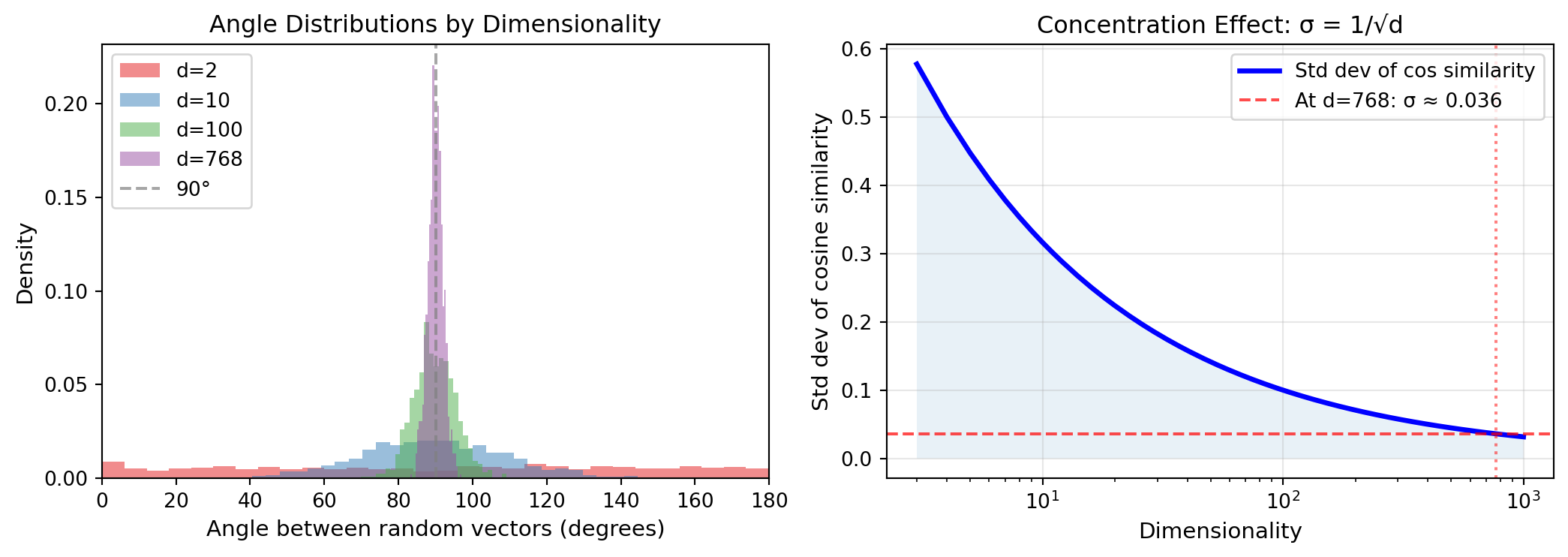
This isn't intuition from low dimensions—it's a mathematical fact. As dimensionality increases, the distribution of angles between random vectors concentrates tightly around 90°.
::: {.callout-note}
## The Math Behind This
The cosine of the angle between two random unit vectors is their dot product. For random vectors, this dot product is approximately normally distributed with mean 0 and variance 1/d (where d is the dimensionality). For d = 768, the standard deviation is about 0.036—angles are almost all between 88° and 92°.
:::
```{python}
#| label: fig-high-dim-angles
#| fig-cap: "As dimensionality increases, angles between random vectors concentrate around 90°. This is why high dimensions enable superposition."
#| code-fold: true
import numpy as np
import matplotlib.pyplot as plt

np.random.seed(42)

fig, (ax1, ax2) = plt.subplots(1, 2, figsize=(11, 4))

# Left plot: Distribution of angles at different dimensionalities
dimensions = [2, 10, 100, 768]
colors = ['#e41a1c', '#377eb8', '#4daf4a', '#984ea3']
n_samples = 1000

for dim, color in zip(dimensions, colors):
    # Generate random unit vectors
    v1 = np.random.randn(n_samples, dim)
    v2 = np.random.randn(n_samples, dim)
    v1 = v1 / np.linalg.norm(v1, axis=1, keepdims=True)
    v2 = v2 / np.linalg.norm(v2, axis=1, keepdims=True)

    # Compute angles in degrees
    cos_sim = np.sum(v1 * v2, axis=1)
    angles = np.arccos(np.clip(cos_sim, -1, 1)) * 180 / np.pi

    ax1.hist(angles, bins=30, alpha=0.5, color=color, label=f'd={dim}', density=True)

ax1.axvline(x=90, color='gray', linestyle='--', alpha=0.7, label='90°')
ax1.set_xlabel('Angle between random vectors (degrees)', fontsize=11)
ax1.set_ylabel('Density', fontsize=11)
ax1.set_title('Angle Distributions by Dimensionality', fontsize=12)
ax1.legend(loc='upper left')
ax1.set_xlim(0, 180)

# Right plot: Standard deviation of cosine similarity vs dimension
dims = np.logspace(0.5, 3, 50).astype(int)
expected_std = 1 / np.sqrt(dims)

ax2.plot(dims, expected_std, 'b-', lw=2.5, label='Std dev of cos similarity')
ax2.axhline(y=0.036, color='red', linestyle='--', alpha=0.7, label='At d=768: σ ≈ 0.036')
ax2.axvline(x=768, color='red', linestyle=':', alpha=0.5)
ax2.fill_between(dims, 0, expected_std, alpha=0.1)
ax2.set_xscale('log')
ax2.set_xlabel('Dimensionality', fontsize=11)
ax2.set_ylabel('Std dev of cosine similarity', fontsize=11)
ax2.set_title('Concentration Effect: σ = 1/√d', fontsize=12)
ax2.legend(loc='upper right')
ax2.grid(True, alpha=0.3)

plt.tight_layout()
plt.show()
```
::: {.callout-tip collapse="true"}
## Interactive Exploration: Near-Orthogonality
Explore how dimensionality affects the concentration of angles between random vectors:
```{ojs}
//| panel: input
viewof dimension = Inputs.range([2, 1000], {value: 768, step: 1, label: "Dimensions:"})
viewof numVectors = Inputs.range([100, 5000], {value: 1000, step: 100, label: "Sample size:"})
```
```{ojs}
// Generate random angles for the selected dimensionality
function generateAngles(d, n) {
  // In high dimensions, cos similarity ~ Normal(0, 1/sqrt(d))
  // Angle = arccos(cos_sim), concentrated around 90°
  const std = 1 / Math.sqrt(d);
  const angles = [];
  for (let i = 0; i < n; i++) {
    // Sample cos similarity from Normal(0, 1/sqrt(d))
    const u1 = Math.random(), u2 = Math.random();
    const z = Math.sqrt(-2 * Math.log(u1)) * Math.cos(2 * Math.PI * u2);
    const cosSim = Math.max(-1, Math.min(1, z * std));
    const angle = Math.acos(cosSim) * 180 / Math.PI;
    angles.push(angle);
  }
  return angles;
}

angles = generateAngles(dimension, numVectors)
meanAngle = angles.reduce((a, b) => a + b, 0) / angles.length
stdAngle = Math.sqrt(angles.map(a => (a - meanAngle) ** 2).reduce((a, b) => a + b, 0) / angles.length)
```
```{ojs}
Plot.plot({
  height: 300,
  marginLeft: 50,
  x: {label: "Angle between random vectors (degrees)", domain: [0, 180]},
  y: {label: "Count"},
  marks: [
    Plot.rectY(angles, Plot.binX({y: "count"}, {x: d => d, fill: "#4daf4a", fillOpacity: 0.7})),
    Plot.ruleX([90], {stroke: "red", strokeDasharray: "4,4", strokeWidth: 2}),
    Plot.ruleX([meanAngle], {stroke: "blue", strokeWidth: 2})
  ]
})
```
```{ojs}
md`**At ${dimension} dimensions:**
- Mean angle: **${meanAngle.toFixed(1)}°** (red dashed line shows 90°, blue shows mean)
- Standard deviation: **${stdAngle.toFixed(1)}°**
- Expected σ of cosine similarity: **${(1/Math.sqrt(dimension)).toFixed(4)}**

*Try sliding to d=2 vs d=768 to see the dramatic concentration effect!*`
```
:::
Why does this matter? Because **orthogonal vectors don't interfere**.
If two features are represented by orthogonal directions, you can detect each independently. The presence of one doesn't affect the detection of the other. They're geometrically *independent*.
And high dimensions give you many nearly-orthogonal directions for free. In 768 dimensions, you can easily pack thousands of approximately-orthogonal directions—far more than 768.
### The Johnson-Lindenstrauss Intuition
This phenomenon has a precise mathematical formulation: the **Johnson-Lindenstrauss lemma**.
The lemma says: for any set of n points in high-dimensional space, you can project them into a much lower-dimensional space (about $\log n$ dimensions) while approximately preserving all pairwise distances.
For our purposes, the implication is: **high-dimensional geometry is robust**. Structure doesn't collapse when you project or when you pack in more features. There's room—geometric room—for far more independent directions than the raw dimension count suggests.
This sets up a phenomenon we'll explore deeply in Chapter 6: **superposition**. Networks represent more features than they have dimensions by exploiting the fact that almost-orthogonal vectors don't interfere much, especially when features rarely co-occur.
## Visualizing the Invisible
We can't see 768 dimensions. But we have tools to glimpse the structure.
### Dimensionality Reduction
Techniques like PCA (Principal Component Analysis), t-SNE, and UMAP project high-dimensional data into 2D or 3D for visualization.
- **PCA** finds the directions of maximum variance and projects onto them. It preserves global structure but may miss local patterns.
- **t-SNE** and **UMAP** preserve local neighborhood structure—nearby points stay nearby. They reveal clusters and separations but can distort global distances.
When you visualize transformer embeddings with t-SNE, you see structure: words cluster by topic, sentences cluster by meaning, similar contexts group together. The clusters are real—they reflect the high-dimensional geometry, partially projected.
But be careful. Dimensionality reduction is lossy. The 2D picture is a shadow of the 768D reality. Clusters that appear separate might overlap in full space. Structure that's invisible in 2D might be clear in full dimensionality.
::: {.callout-tip}
## A Practical Tip
Use dimensionality reduction for exploration, not conclusion. If you see a pattern in t-SNE, verify it with linear probes or direct cosine similarity in the original space. The visualization is a starting point, not proof.
:::
### Direct Geometric Analysis
For more rigorous analysis, work in the full-dimensional space:
- Compute cosine similarities between specific vectors
- Project representations onto hypothesized feature directions
- Measure clustering with silhouette scores or other metrics
- Use linear classifiers to test if properties are linearly separable
The geometry is there whether or not you can visualize it. The tools work in full dimensionality.
## What the Geometry Enables
Let's connect this back to mechanistic interpretability.
### Attribution via Projection
The residual stream is a sum of contributions from attention heads and MLPs (Chapter 3). Each contribution is a vector. To understand how much a component contributed to a particular prediction, we can project its output onto the direction of that prediction.
If an attention head writes a vector that points strongly toward "Paris" in vocabulary space, that head is contributing to predicting "Paris." The geometry makes attribution possible: direction tells you what each component is "saying."
### Feature Detection via Linear Classifiers
If we hypothesize that the model has a "code" feature (does this text look like code?), we can train a linear probe to detect it. A successful probe means: there's a hyperplane in activation space that separates "code" from "not code."
Finding the hyperplane reveals the feature direction. Projecting any activation onto that direction tells you how much "code-ness" the model detects.
### Intervention via Vector Arithmetic
If you know the "truthfulness" direction, you can add to it and make the model more truthful (or subtract and make it less). If you know the "Golden Gate Bridge" direction, you can amplify it and make the model obsess over bridges.
This isn't magic—it's geometry. Directions encode features. Modifying vectors along those directions modifies the encoded features. The linear structure makes intervention predictable.
## Limits of the Geometric View
The geometric perspective is powerful but not perfect.
### Not Everything is Linear
Some features may not be linearly encoded. Complex combinations of concepts might live in curved manifolds or require nonlinear detection. The linear representation hypothesis is a working assumption, not a proven law.
### Geometry Doesn't Tell You "Why"
Knowing that two concepts point in similar directions doesn't explain *why* the network learned to represent them that way. Geometry is descriptive, not explanatory. Understanding the mechanism requires going beyond geometry to circuits and algorithms.
### The Basis Problem
A direction is a line through the origin. But which direction corresponds to which feature? The network doesn't label its directions. We have to discover them through probing, intervention, and interpretation.
This is harder than it sounds. In 768 dimensions, there are infinitely many directions. Most mean nothing. Finding the meaningful ones—the ones that correspond to human-interpretable features—is an open research problem.
::: {.callout-important}
## The Core Challenge
The geometry gives us a framework. Activations are vectors. Features are directions. Similarity is proximity. But we still need to find *which* directions matter—which ones correspond to the features the network actually uses. This is the project of mechanistic interpretability.
:::
## Polya's Perspective: Building Intuition Before Formalism
This chapter is an exercise in Polya's heuristic: **understand the problem before solving it**.
We haven't yet defined "features" precisely—that's Chapter 5. We haven't explained superposition—that's Chapter 6. We haven't given you tools to find circuits—that's Arc III.
But we've built geometric intuition. Now when we say "a feature is a direction in activation space," you understand what that means. When we say "features are superimposed because high dimensions allow near-orthogonality," you have the geometric background.
This is Polya's approach: introduce concepts intuitively before formalizing them. The geometry is the intuition; the features and circuits are the formalism.
::: {.callout-tip}
## Polya's Heuristic: Draw a Figure
Polya emphasized visualization: "Draw a figure. Introduce suitable notation." We can't draw 768-dimensional figures, but we can:
1. Reason about 2D/3D analogies carefully
2. Use dimensionality reduction for exploration
3. Work with linear algebra (projections, dot products, angles) to query the geometry directly
The figure is implicit, but the geometric reasoning is explicit.
:::
## Looking Ahead
We've established that the residual stream has geometric structure: distance reflects similarity, direction reflects properties, high dimensions enable rich representations.
But we've been vague about what the important directions *are*. We've talked about "features" without defining them. We've assumed directions correspond to human-interpretable concepts without explaining why or how to find them.
The next chapter tackles this directly: **What exactly is a feature?**
::: {.callout-note}
## A Mystery to Solve
Here's something surprising: Anthropic found over 2 million interpretable features in a model with only 4,096 dimensions. That's 500 features per dimension. If features are directions, and you can only have as many orthogonal directions as dimensions... how is this possible?
The answer, which we'll explore in Chapter 6, involves a beautiful piece of geometry that explains both why neural networks are so powerful and why they're so hard to interpret.
:::
Here's the question to carry forward: if the network represents more concepts than it has dimensions (because almost-orthogonal directions don't interfere), how do we untangle them? How do we find the directions that matter? And what happens when the directions *do* interfere—when the model's capacity is pushed to its limits?
The geometry gives us the framework. Now we need to find the atoms of meaning within it.
---
## Key Takeaways
::: {.callout-tip}
## 📋 Summary Card
```
┌────────────────────────────────────────────────────────────┐
│  ACTIVATIONS AS GEOMETRY                                   │
├────────────────────────────────────────────────────────────┤
│                                                            │
│  CORE INSIGHT:   Activations are points in high-dim space  │
│                  Features are DIRECTIONS, not neurons      │
│                                                            │
│  KEY PROPERTIES:                                           │
│    • Distance → semantic similarity                        │
│    • Direction → semantic properties (gender, royalty...)  │
│    • Cosine similarity → how related two concepts are      │
│                                                            │
│  LINEAR REPRESENTATION HYPOTHESIS:                         │
│    Properties are encoded as linear directions             │
│    → Enables probing, steering, interpretation             │
│                                                            │
│  HIGH-DIM SURPRISE:                                        │
│    Random vectors are ~90° apart (nearly orthogonal)       │
│    → Can pack MANY more features than dimensions           │
│    → Foundation for superposition (Chapter 6)              │
│                                                            │
└────────────────────────────────────────────────────────────┘
```
:::
## Check Your Understanding
::: {.callout-note collapse="true"}
## Question 1: Why does "king - man + woman ≈ queen" work?
**Answer**: Because semantic properties like gender are encoded as *consistent directions* in the embedding space. The vector from "man" to "woman" represents the "gender direction." This same direction, when applied to "king," moves it to "queen" because the direction is consistent across different concepts. This is evidence for the **linear representation hypothesis**—that semantic properties correspond to linear directions in activation space.
:::
::: {.callout-note collapse="true"}
## Question 2: Why do random vectors in high dimensions tend to be nearly perpendicular?
**Answer**: As dimensionality increases, the dot product between random unit vectors (which equals the cosine of the angle between them) has a distribution that concentrates around zero with variance 1/d. For d=768, the standard deviation is only ~0.036, meaning angles are almost always between 88° and 92°. This is a mathematical consequence of high-dimensional geometry, not intuition from 2D/3D. It's crucial because **orthogonal vectors don't interfere**—this property enables superposition.
:::
::: {.callout-note collapse="true"}
## Question 3: What does it mean to "project onto a feature direction" and why is it useful?
**Answer**: Projecting a vector onto a feature direction computes the dot product between the activation vector and the unit vector representing that feature. The result tells you **how strongly that feature is present** in the activation. For example, if you know the "truthfulness" direction, projecting any activation onto it tells you how much "truthfulness" the model is encoding at that point. This is useful for:
1. **Feature detection**: Check if a property is present
2. **Attribution**: Measure how much a component contributed to a prediction
3. **Intervention**: Add to or subtract from feature directions to steer behavior
:::
---
## Further Reading
1. **Word2Vec Explained** — [Towards Data Science](https://towardsdatascience.com/word2vec-explained-49c52b4ccb71): Accessible introduction to word embeddings and the king - man + woman = queen phenomenon.
2. **On the Origins of Linear Representations in Large Language Models** — [arXiv:2403.03867](https://arxiv.org/abs/2403.03867): Recent research showing linear structure persists beyond embeddings into transformer hidden layers.
3. **Toy Models of Superposition** — [Anthropic](https://transformer-circuits.pub/2022/toy_model/index.html): The foundational paper on how high-dimensional geometry enables superposition. Essential reading for Chapter 6.
4. **Neural Networks, Manifolds, and Topology** — [Chris Olah](https://colah.github.io/posts/2014-03-NN-Manifolds-Topology/): Classic blog post on how neural networks learn to disentangle data through geometric transformations.
5. **Probing Classifiers: Promises, Shortcomings, and Advances** — [Computational Linguistics](https://direct.mit.edu/coli/article/48/1/207/107571/Probing-Classifiers-Promises-Shortcomings-and): Critical perspective on linear probing—what it shows and what it doesn't.
6. **The Johnson-Lindenstrauss Lemma** — [Number Analytics](https://www.numberanalytics.com/blog/johnson-lindenstrauss-lemma-computational-geometry): Intuitive explanation of the mathematical foundations of high-dimensional geometry.