---
title: "The Superposition Hypothesis"
subtitle: "Why interpretability is fundamentally hard"
author: "Taras Tsugrii"
date: 2025-01-05
categories: [core-theory, superposition]
description: "Neural networks represent far more features than they have dimensions. This compression scheme—superposition—is why polysemanticity exists and why mechanistic interpretability is hard."
---
::: {.callout-tip}
## What You'll Learn
- Why networks can pack more features than dimensions
- The geometry of "almost orthogonal" and why it enables compression
- How superposition creates polysemanticity
- The phase transition between superposed and dedicated representations
:::
::: {.callout-warning}
## Prerequisites
**Required**: [Chapter 5: Features](05-features.qmd) — understanding what features are and why neurons are polysemantic
:::
::: {.callout-note}
## Before You Read: Recall
From Chapter 5, recall:
- Features are *directions* in activation space, not individual neurons
- Neurons are polysemantic (respond to multiple unrelated concepts)
- The goal: decompose polysemantic neurons into monosemantic features
- Evidence for linear representations: steering works, vector arithmetic works
**Now we ask**: How do networks fit thousands of features into hundreds of dimensions?
:::
## The Capacity Puzzle
In the previous chapter, we established that features are directions in activation space. A 768-dimensional residual stream can represent features as directions—unit vectors pointing in meaningful orientations.
Here's the puzzle: how many directions can you fit in 768 dimensions?
Naively, the answer is 768. You can have 768 orthogonal directions—that's what "768-dimensional" means. Each direction is perpendicular to all others, so they don't interfere. Clean, simple, interpretable.
But when Anthropic researchers analyzed Claude 3 Sonnet's activations, they found something startling: **over 2 million interpretable features** in a single 4,096-dimensional layer. That's a ratio of roughly 500 features per dimension.
This isn't a mistake. This is **superposition**—the central phenomenon that makes neural networks both powerful and hard to interpret.
::: {.callout-note}
## The Core Claim
The superposition hypothesis states that neural networks encode far more features than they have dimensions by storing multiple sparse features in overlapping representations. The features are *almost* orthogonal—close enough that interference is manageable when features rarely co-occur.
:::
This chapter explains what superposition is, why it works, and why it's the fundamental obstacle to mechanistic interpretability.
## The Efficiency Argument
Why would a network use superposition? Because it's efficient.
Consider a language model that needs to represent millions of concepts: every word, every grammatical pattern, every fact about the world, every style of writing, every domain of knowledge. If each concept required a dedicated dimension, you'd need a model with millions of dimensions per layer.
But here's the key observation: **most features are sparse**.
- The "French" feature activates on maybe 2% of text
- The "cooking" feature activates on maybe 3% of text
- The "Golden Gate Bridge" feature activates on maybe 0.05% of text
- Most specialized features activate on less than 0.1% of inputs
At any given moment, only a tiny fraction of features are active. The model doesn't need to represent all features simultaneously—it just needs to represent the few that matter for the current input.
This creates an opportunity. If features rarely co-occur, you can pack them into overlapping representations. The overlap only causes problems when multiple superimposed features activate together—which, by assumption, is rare.
::: {.callout-tip}
## A Performance Engineering Parallel
Superposition is like memory overcommitment in operating systems. The OS promises more virtual memory than physical RAM exists, betting that not all processes will use their full allocation simultaneously. Most of the time, this works. Occasionally, you get swapping. Neural networks make the same bet: pack more features than dimensions, accept occasional interference.
:::
## The Geometry of Almost-Orthogonal
How does superposition actually work geometrically?
In Chapter 4, we noted that high-dimensional spaces have a surprising property: random vectors are almost always nearly perpendicular. In 768 dimensions, two random unit vectors have a dot product with standard deviation of about 0.036—their angle is almost certainly between 88° and 92°.
This is the geometric foundation of superposition. You don't need features to be *perfectly* orthogonal. You just need them to be *almost* orthogonal—close enough that interference is small.
### The Interference Trade-off
When two features have directions with cosine similarity $c$ (where $c = 0$ is orthogonal and $c = 1$ is parallel), their interference cost is roughly proportional to $c^2$.
- Cosine similarity 0.05 → 0.25% interference
- Cosine similarity 0.1 → 1% interference
- Cosine similarity 0.3 → 9% interference
Small deviations from orthogonality have small costs. This is why superposition works: you can pack thousands of features with cosine similarities around 0.03-0.05, and the interference remains manageable.
### Packing More Than Dimensions
Here's the mathematical punch line: in $d$ dimensions, you can fit roughly $e^{O(d)}$ almost-orthogonal vectors—exponentially more than $d$.
This isn't just theoretical. The Johnson-Lindenstrauss lemma, which we mentioned in Chapter 4, guarantees that high-dimensional projections approximately preserve distances. The same mathematics applies here: high-dimensional spaces have *far more room* for nearly-independent directions than low-dimensional intuition suggests.
A 768-dimensional space can comfortably hold tens of thousands of nearly-orthogonal directions. A 4,096-dimensional space can hold millions. This is why superposition is so effective—the geometry allows it.
::: {.callout-warning}
## Pause and Think
If superposition lets networks pack many features into limited dimensions, why is this a problem for interpretability?
*Hint*: Think about what happens when you look at a single neuron's activation.
:::
## Polytope Arrangements
When researchers study superposition in toy models, they find that networks don't just pack features randomly. They arrange them with elegant geometric structure.
Consider a minimal case: representing 4 sparse features in 2 dimensions. You can't fit 4 orthogonal directions in 2D (only 2 are possible). But you *can* arrange 4 directions as the corners of a square:
```
       Feature 2
           ↑
           |
Feature 1 ←+→ Feature 3
           |
           ↓
       Feature 4
```
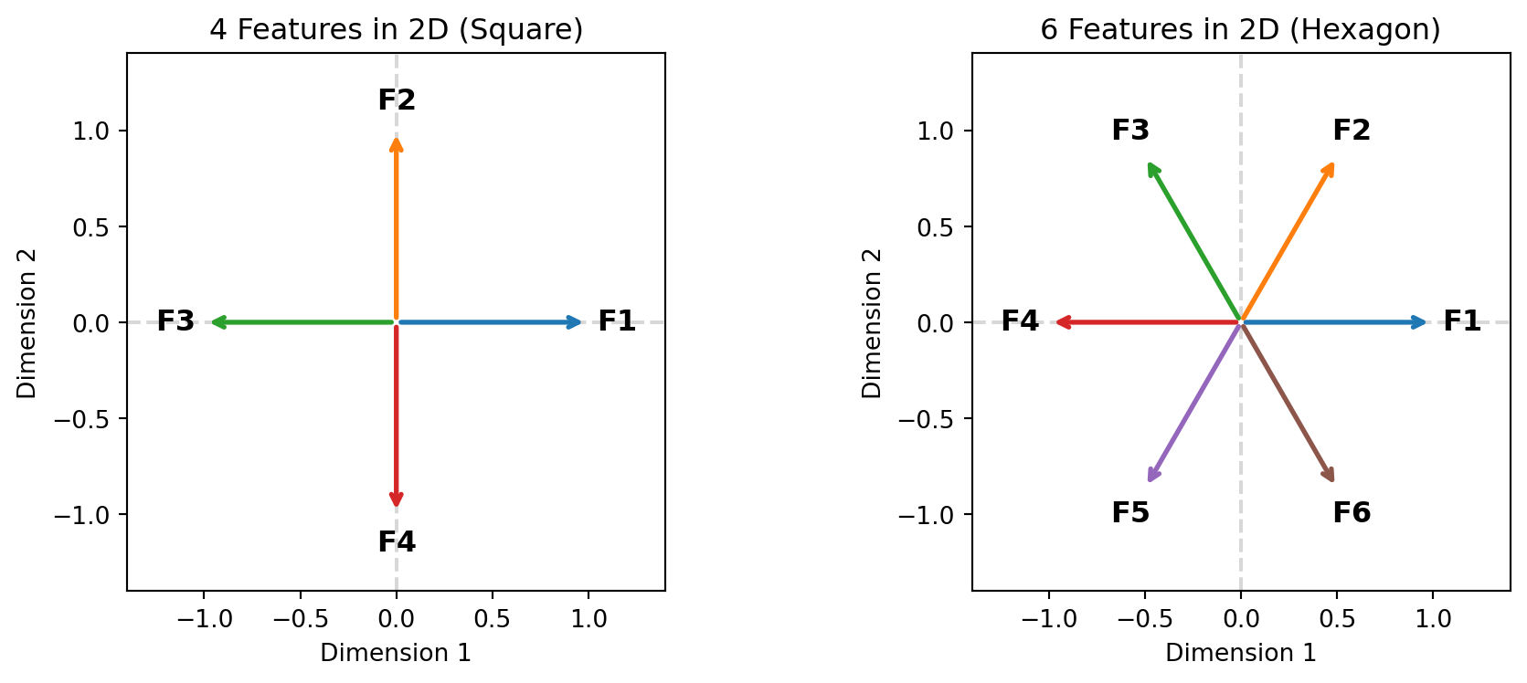
Here's what this looks like geometrically—4 features arranged as a square, and 6 features arranged as a hexagon:
```{python}
#| label: fig-polytopes
#| fig-cap: "Optimal arrangements for features in 2D: 4 features form a square (left), 6 features form a hexagon (right). Each feature is a direction (arrow) from the origin."
#| code-fold: true
import numpy as np
import matplotlib.pyplot as plt

fig, (ax1, ax2) = plt.subplots(1, 2, figsize=(10, 4))

# 4 features as a square
angles_4 = np.linspace(0, 2*np.pi, 5)[:-1]  # 0, 90, 180, 270 degrees
for i, angle in enumerate(angles_4):
    ax1.annotate('', xy=(np.cos(angle), np.sin(angle)), xytext=(0, 0),
                arrowprops=dict(arrowstyle='->', color=f'C{i}', lw=2))
    ax1.text(1.15*np.cos(angle), 1.15*np.sin(angle), f'F{i+1}',
             ha='center', va='center', fontsize=12, fontweight='bold')

ax1.set_xlim(-1.4, 1.4)
ax1.set_ylim(-1.4, 1.4)
ax1.set_aspect('equal')
ax1.axhline(y=0, color='gray', linestyle='--', alpha=0.3)
ax1.axvline(x=0, color='gray', linestyle='--', alpha=0.3)
ax1.set_title('4 Features in 2D (Square)', fontsize=12)
ax1.set_xlabel('Dimension 1')
ax1.set_ylabel('Dimension 2')

# 6 features as a hexagon
angles_6 = np.linspace(0, 2*np.pi, 7)[:-1]  # 60-degree spacing
for i, angle in enumerate(angles_6):
    ax2.annotate('', xy=(np.cos(angle), np.sin(angle)), xytext=(0, 0),
                arrowprops=dict(arrowstyle='->', color=f'C{i}', lw=2))
    ax2.text(1.15*np.cos(angle), 1.15*np.sin(angle), f'F{i+1}',
             ha='center', va='center', fontsize=12, fontweight='bold')

ax2.set_xlim(-1.4, 1.4)
ax2.set_ylim(-1.4, 1.4)
ax2.set_aspect('equal')
ax2.axhline(y=0, color='gray', linestyle='--', alpha=0.3)
ax2.axvline(x=0, color='gray', linestyle='--', alpha=0.3)
ax2.set_title('6 Features in 2D (Hexagon)', fontsize=12)
ax2.set_xlabel('Dimension 1')
ax2.set_ylabel('Dimension 2')

plt.tight_layout()
plt.show()
```
Each pair of adjacent features is at 90°—perfectly orthogonal. Each pair of opposite features is at 180°—maximally separated. This is the optimal arrangement for 4 features in 2D.
For 6 features in 2D, the optimal arrangement is a regular hexagon. For more features, you get regular polytopes (higher-dimensional generalizations of polygons). The network learns to maximize the minimum angle between any two features, minimizing worst-case interference.
::: {.callout-note}
## Emergent Structure
Networks discover these polytope arrangements through gradient descent, not through explicit programming. The geometry is optimal, and optimization finds it. This suggests superposition isn't an accident—it's the natural solution to the problem of representing sparse features in limited dimensions.
:::
::: {.callout-note}
## The Discovery Story
In 2022, researchers at Anthropic—including Shan Carter, Chris Olah, and Nelson Elhage—were trying to understand why neural networks are so hard to interpret. They built the simplest possible toy model: a tiny autoencoder with more features than dimensions. What they observed was striking: the network didn't just randomly arrange features. It discovered regular polytopes—pentagons, hexagons, and their higher-dimensional cousins. The paper, "Toy Models of Superposition," became one of the foundational works in mechanistic interpretability, showing that superposition isn't chaos—it's elegant geometry.
:::
## How Superposition Creates Polysemanticity
Now we can explain the polysemantic neuron from Chapter 5—the one that activated for cat faces *and* car fronts.
In a world without superposition:
- The "cat face" feature would have its own dedicated neurons
- The "car front" feature would have its own dedicated neurons
- Each neuron would be monosemantic
In a world with superposition:
- The "cat face" feature is a direction in activation space
- The "car front" feature is a different direction
- These directions are *almost* orthogonal—say, 87° apart
- Both directions pass through some of the same neurons
- When you look at neuron 847, it participates in both directions
- Neuron 847 activates for cat faces *and* car fronts
The neuron is polysemantic because it's the intersection of multiple feature directions. Each feature, as a direction, is monosemantic. But the neuron, as a point where multiple directions overlap, appears polysemantic.
::: {.callout-important}
## The Key Insight
Polysemanticity is a *symptom* of superposition, not a separate phenomenon. The network is packing multiple monosemantic features into overlapping representations. Individual neurons look confusing because they're the cross-section of a higher-dimensional structure we can't see directly.
:::
::: {.callout-caution}
## Common Misconception: Superposition Means Features Are "Mixed"
**Wrong**: "In superposition, the model can't distinguish between features—they're blended together."
**Right**: Features remain distinct directions. The model *can* distinguish them via their direction, even if individual neurons respond to multiple features. It's like separating sounds by frequency: each sound is still there, just overlapping in time. Superposition encodes cleanly; *we* have trouble reading it because we look at neurons instead of directions.
:::
## The Sparsity Requirement
Superposition only works when features are sparse. Here's why.
If two features with cosine similarity 0.1 both activate simultaneously, you get 1% interference. Not great, but manageable.
But if they *always* activate simultaneously, you *always* get that interference. The "features" become indistinguishable—the network can't tell them apart.
Sparsity makes superposition viable:
- Feature A activates 2% of the time
- Feature B activates 3% of the time
- If independent, they co-occur only 0.06% of the time
- Interference happens rarely → superposition is worth it
The sparser the features, the more you can superimpose. This is why models can pack millions of features: most real-world concepts are rare enough that their co-occurrence is negligible.
### What Happens at High Density?
When features become less sparse (more frequently active), superposition becomes less beneficial:
- At 50% activation (not sparse at all), interference is constant
- The cost of packing outweighs the benefit
- Networks allocate dedicated capacity instead
This creates a **phase transition**: as sparsity crosses a threshold, the optimal representation strategy suddenly changes from superimposed to dedicated.
## Phase Transitions
The phase transition is one of the most striking findings from superposition research.
In toy models, researchers can control the sparsity of features and observe what representation the network learns. Here's what happens:
**High sparsity (rare features)**:
- Network uses heavy superposition
- Features arranged as polytope vertices
- Many more features than dimensions
- High compression, occasional interference
**Critical sparsity threshold**:
- Sharp transition
- Representation structure changes qualitatively
- Loss drops or jumps suddenly
**Low sparsity (common features)**:
- Network uses minimal superposition
- Features get dedicated dimensions
- Fewer features than could fit
- Clean representation, no interference
The transition is *sharp*, not gradual. Small changes in sparsity near the threshold cause large changes in learned representation.
::: {.callout-tip}
## Why Phase Transitions Matter
Phase transitions tell us that superposition isn't a dial—it's a switch. Networks either use superposition heavily or barely at all, depending on the sparsity of their features. Understanding where real models sit relative to the threshold helps us understand how hard interpretation will be.
:::
Modern language models appear to operate deep in the high-sparsity regime. Their features are sparse enough that superposition is heavily advantageous. This is why they can represent millions of features in thousands of dimensions—and why they're so hard to interpret.
## Interactive: Explore Feature Packing
Use the sliders below to explore how features pack into limited dimensions. The **interference meter** shows how problematic co-activation would be at different sparsity levels. Click **Simulate Activations** to see random feature activations based on the probability.
```{ojs}
//| label: fig-superposition-interactive
//| fig-cap: "Interactive visualization of superposition. Adjust features and sparsity, then simulate to see interference in action."
viewof numFeatures = Inputs.range([2, 12], {step: 1, value: 4, label: "Number of features"})
viewof sparsity = Inputs.range([0.01, 0.5], {step: 0.01, value: 0.05, label: "Activation probability"})
viewof simulateBtn = Inputs.button("Simulate Activations")

dimensions = 2

// Calculate feature directions (evenly spaced around circle)
featureAngles = Array.from({length: numFeatures}, (_, i) => (2 * Math.PI * i) / numFeatures)
featureVectors = featureAngles.map(a => ({x: Math.cos(a), y: Math.sin(a)}))

// Calculate worst-case interference (max cosine similarity between non-identical pairs)
worstInterference = {
  if (numFeatures <= 2) return 0;
  const angle = (2 * Math.PI) / numFeatures;
  return Math.abs(Math.cos(angle));
}

// Expected co-occurrence probability
cooccurrence = sparsity * sparsity

// Effective interference (probability-weighted)
effectiveInterference = worstInterference * cooccurrence * numFeatures

// Simulate which features are active (re-runs when button clicked or sparsity changes)
activeFeatures = {
  simulateBtn;  // Dependency on button
  return Array.from({length: numFeatures}, () => Math.random() < sparsity);
}

// Count active and check for interference
numActive = activeFeatures.filter(x => x).length
hasInterference = numActive >= 2

// Visualization with two panels
{
  const width = 700;
  const height = 400;
  const radius = 140;

  const svg = d3.create("svg")
    .attr("viewBox", [0, 0, width, height])
    .attr("width", width)
    .attr("height", height);

  // Left panel: Feature directions
  const leftG = svg.append("g").attr("transform", `translate(180, 200)`);

  // Background circle
  leftG.append("circle")
    .attr("r", radius)
    .attr("fill", "none")
    .attr("stroke", "#ddd")
    .attr("stroke-width", 1);

  // Axes
  leftG.append("line").attr("x1", -radius).attr("y1", 0).attr("x2", radius).attr("y2", 0).attr("stroke", "#ddd");
  leftG.append("line").attr("x1", 0).attr("y1", -radius).attr("x2", 0).attr("y2", radius).attr("stroke", "#ddd");

  // Title
  leftG.append("text").attr("y", -radius - 20).attr("text-anchor", "middle").attr("font-size", "14px").attr("font-weight", "bold").text("Feature Directions");

  // Feature arrows
  const colors = d3.schemeTableau10;
  featureVectors.forEach((v, i) => {
    const isActive = activeFeatures[i];
    leftG.append("line")
      .attr("x1", 0).attr("y1", 0)
      .attr("x2", v.x * radius * 0.85).attr("y2", -v.y * radius * 0.85)
      .attr("stroke", colors[i % 10])
      .attr("stroke-width", isActive ? 5 : 2)
      .attr("opacity", isActive ? 1 : 0.3)
      .attr("marker-end", "url(#arrow)");

    leftG.append("text")
      .attr("x", v.x * radius * 1.0)
      .attr("y", -v.y * radius * 1.0)
      .attr("text-anchor", "middle")
      .attr("font-size", isActive ? "14px" : "11px")
      .attr("font-weight", isActive ? "bold" : "normal")
      .attr("fill", colors[i % 10])
      .attr("opacity", isActive ? 1 : 0.5)
      .text(`F${i + 1}`);
  });

  // Arrow marker
  svg.append("defs").append("marker")
    .attr("id", "arrow")
    .attr("viewBox", "0 -5 10 10")
    .attr("refX", 8)
    .attr("markerWidth", 6)
    .attr("markerHeight", 6)
    .attr("orient", "auto")
    .append("path")
    .attr("d", "M0,-5L10,0L0,5")
    .attr("fill", "#666");

  // Right panel: Interference meter
  const rightG = svg.append("g").attr("transform", `translate(500, 80)`);

  rightG.append("text").attr("text-anchor", "middle").attr("font-size", "14px").attr("font-weight", "bold").text("Interference Risk");

  // Meter background
  const meterWidth = 30;
  const meterHeight = 200;
  rightG.append("rect")
    .attr("x", -meterWidth/2)
    .attr("y", 20)
    .attr("width", meterWidth)
    .attr("height", meterHeight)
    .attr("fill", "#eee")
    .attr("stroke", "#999")
    .attr("rx", 4);

  // Meter fill (based on effective interference, scaled)
  const meterLevel = Math.min(1, effectiveInterference * 5);  // Scale for visibility
  const fillColor = meterLevel < 0.3 ? "#4CAF50" : meterLevel < 0.6 ? "#FFC107" : "#f44336";
  rightG.append("rect")
    .attr("x", -meterWidth/2 + 2)
    .attr("y", 20 + meterHeight * (1 - meterLevel))
    .attr("width", meterWidth - 4)
    .attr("height", meterHeight * meterLevel)
    .attr("fill", fillColor)
    .attr("rx", 2);

  // Labels
  rightG.append("text").attr("x", meterWidth/2 + 8).attr("y", 30).attr("font-size", "10px").attr("fill", "#666").text("High");
  rightG.append("text").attr("x", meterWidth/2 + 8).attr("y", 130).attr("font-size", "10px").attr("fill", "#666").text("Med");
  rightG.append("text").attr("x", meterWidth/2 + 8).attr("y", 220).attr("font-size", "10px").attr("fill", "#666").text("Low");

  // Status text
  const statusY = 260;
  rightG.append("text")
    .attr("y", statusY)
    .attr("text-anchor", "middle")
    .attr("font-size", "12px")
    .attr("fill", hasInterference ? "#f44336" : "#4CAF50")
    .attr("font-weight", "bold")
    .text(hasInterference ? `⚠ ${numActive} features active!` : numActive === 1 ? "✓ 1 feature active" : "○ No features active");

  rightG.append("text")
    .attr("y", statusY + 18)
    .attr("text-anchor", "middle")
    .attr("font-size", "11px")
    .attr("fill", "#666")
    .text(hasInterference ? "Interference occurring" : "No interference");

  return svg.node();
}
```
```{ojs}
//| echo: false
html`<div style="background: #f8f9fa; padding: 1rem; border-radius: 8px; margin: 1rem 0;">
<strong>Analysis:</strong><br>
• <strong>Features</strong>: ${numFeatures} packed into ${dimensions} dimensions<br>
• <strong>Angle between adjacent features</strong>: ${(360 / numFeatures).toFixed(1)}° ${360/numFeatures >= 90 ? "(orthogonal)" : 360/numFeatures >= 60 ? "(good separation)" : "(crowded)"}<br>
• <strong>Geometric interference</strong> (cosine similarity): ${(worstInterference * 100).toFixed(1)}%<br>
• <strong>Co-occurrence probability</strong> (at ${(sparsity*100).toFixed(0)}% activation): ${(cooccurrence * 100).toFixed(2)}%<br>
• <strong>Expected total interference</strong>: ${effectiveInterference < 0.05 ? "✓ Low — superposition works well" : effectiveInterference < 0.15 ? "⚠ Moderate — acceptable trade-off" : "✗ High — consider fewer features"}<br><br>
<em>The key insight: even with high geometric interference, low activation probability keeps expected interference manageable.</em>
</div>`
```
::: {.callout-note}
## Key Insight
Notice how adding more features decreases the angle between them (increasing interference), but if sparsity is low enough (features rarely activate), the expected interference remains manageable. This is the superposition trade-off in action.
:::
## Evidence for Superposition
Is superposition real, or just a theoretical possibility? The evidence is strong.
### Toy Model Experiments
The foundational work by Anthropic (2022) trained simple networks to store sparse features explicitly. The findings:
- Networks consistently learned superposed representations
- Feature directions matched theoretically optimal polytope arrangements
- Interference patterns matched predictions
- Phase transitions occurred at predicted sparsity thresholds
### Scaling Monosemanticity
When Anthropic applied sparse autoencoders to Claude 3 Sonnet (2024), they found:
- Over 2 million interpretable features in one layer
- Features were sparse (most activate < 0.1% of the time)
- Features were monosemantic (each corresponds to one concept)
- Features had causal power (manipulating them changed behavior)
This is only possible if the original activations were superposed. The sparse autoencoder is *decomposing* superposition into individual features.
### Cross-Modal Transfer
The "Golden Gate Bridge" feature, discovered on text, also activated on images of the bridge—even though the model was trained only on text. This transfer only makes sense if the feature is a genuine direction in activation space, not an artifact of specific neurons.
### Steering Experiments
Adding feature directions to activations shifts model behavior predictably. The "honesty" direction makes models more honest. The "refusal" direction makes them refuse more. This works because features are linear directions, exactly as superposition predicts.
## Why This Makes Interpretation Hard
Superposition is the fundamental obstacle to mechanistic interpretability. Here's why.
### The Alignment Problem
The network's natural basis (neurons) is misaligned with the features' natural basis (superposed directions). When you look at a neuron, you see a confusing mix of unrelated concepts. When you look at activations, you see a superposition of many features.
To interpret the network, you have to *undo* the superposition—find the monosemantic directions hidden in the polysemantic neurons. This is computationally expensive and conceptually difficult.
### The Haystack Problem
In a 768-dimensional space with potentially millions of features, finding a specific feature is like finding a needle in a haystack the size of a stadium. Which direction corresponds to "truthfulness"? Which to "code quality"? Which to "French cuisine"?
There's no label. You have to discover features through probing, pattern matching, and verification—one at a time.
### Interference Noise
Even when you find a feature, its signal is noisy. Other superimposed features add interference. Distinguishing "this activation is strongly feature A with weak feature B interference" from "this activation is weakly feature A with no interference" is genuinely hard.
### The Scale Problem
Modern models have:
- Hundreds of layers
- Thousands of dimensions per layer
- Millions of features per layer
- Different features at different layers
Fully interpreting a frontier model would require discovering and cataloging billions of features. Current tools can handle thousands. The gap is enormous.
::: {.callout-important}
## The Core Challenge
Superposition transforms the interpretation problem from "read the neurons" to "decompose a compressed representation into its component features." This is much harder. It's the difference between reading a file and decompressing a heavily compressed archive whose compression scheme you don't fully understand.
:::
## Limits and Open Questions
Superposition isn't universal. There are exceptions and unknowns.
### When Superposition Doesn't Apply
- **Very common features** (activation > 30-50%) may get dedicated dimensions
- **Safety-critical features** may be encoded more cleanly for reliability
- **Very large models** may have enough capacity to avoid superposition for some features
### Incidental Polysemanticity
Recent research shows polysemanticity can emerge even without capacity pressure. Networks sometimes assign multiple features to the same neuron purely due to initialization and training dynamics. This suggests superposition isn't the *only* cause of polysemanticity—though it's probably the primary cause.
### The Ontology Question Redux
We still don't know if the features we discover through sparse autoencoders are the network's "natural" features or artifacts of our analysis method. Superposition makes this harder: there are infinitely many ways to decompose a superposed representation, and we might be finding our preferred decomposition rather than the network's.
### Do Very Large Models Escape?
An open question: as models scale to trillions of parameters, do they eventually have enough capacity that superposition becomes unnecessary? Or does the number of features scale with model size, maintaining the pressure? Current evidence suggests the latter, but it's not certain.
## Polya's Perspective: Understanding the Obstacle
In Polya's framework, we've now understood why the problem is hard.
Chapter 1: What are we trying to do? (Reverse engineer the algorithm.)
Chapters 2-4: What's the substrate? (Matrix multiplication in a geometric space.)
Chapter 5: What are we looking for? (Features—directions in that space.)
Chapter 6: What's the obstacle? (**Superposition—features are packed densely, hiding in polysemantic neurons.**)
This is Polya's approach: before devising a solution, fully understand the difficulty. Superposition isn't just a nuisance; it's a fundamental property of how neural networks compress information. Any successful interpretation method must deal with it.
::: {.callout-tip}
## Polya's Heuristic: What Makes This Hard?
Good problem-solving requires understanding *why* a problem is difficult, not just *that* it's difficult. Superposition tells us: the difficulty is compression. The network has encoded exponentially more features than it has dimensions, and we have to decompress.
:::
## Looking Ahead
We've established that superposition is why interpretation is hard. But can we study superposition in a controlled setting? Can we build a model simple enough to fully understand, that still exhibits superposition?
Yes. The next chapter covers **toy models**—simplified networks that exhibit superposition clearly and completely. By studying these toy models, we can verify our understanding, build intuition, and prepare for the messier reality of real networks.
This is Polya's heuristic in action: **solve a simpler problem first**. If we can understand superposition in a 2-dimensional network with 5 features, we're better prepared to understand it in a 4,096-dimensional network with 2 million features.
---
## Key Takeaways
::: {.callout-tip}
## 📋 Summary Card
```
┌────────────────────────────────────────────────────────────┐
│  THE SUPERPOSITION HYPOTHESIS                              │
├────────────────────────────────────────────────────────────┤
│                                                            │
│  WHAT IT IS:    Networks pack MORE features than dimensions│
│                 by using almost-orthogonal directions      │
│                                                            │
│  WHY IT WORKS:                                             │
│    • Sparse features rarely co-occur                       │
│    • Almost-orthogonal ≈ low interference                  │
│    • High-dim spaces have MANY near-orthogonal directions  │
│                                                            │
│  THE CONSEQUENCE:                                          │
│    Polysemanticity = neurons participate in MULTIPLE       │
│    feature directions → look confusing when examined       │
│                                                            │
│  WHY IT'S HARD:                                            │
│    • Neuron basis ≠ feature basis (misaligned)             │
│    • Must decompose compressed representations             │
│    • Millions of features to discover                      │
│                                                            │
│  KEY FINDING:    Phase transition at sparsity threshold    │
│                  Superposition switches on/off sharply     │
│                                                            │
└────────────────────────────────────────────────────────────┘
```
:::
## Check Your Understanding
::: {.callout-note collapse="true"}
## Question 1: Why does a neuron activate for "cat faces" AND "car fronts"?
**Answer**: The neuron is polysemantic because it sits at the intersection of multiple superimposed feature directions. The "cat face" feature is one direction in activation space, and the "car front" feature is a different (but not perfectly orthogonal) direction. Both directions pass through this neuron's activation axis. When either feature is present, the neuron activates. The neuron isn't confused—it's just a cross-section of a higher-dimensional structure where multiple meaningful directions overlap.
:::
::: {.callout-note collapse="true"}
## Question 2: Why is sparsity essential for superposition to work?
**Answer**: Superposition introduces interference when multiple features activate simultaneously. If two features with cosine similarity 0.1 both activate, you get ~1% interference. If they always activated together, you'd always have that interference, and the features would become indistinguishable.
But if Feature A activates 2% of the time and Feature B activates 3% of the time (and independently), they only co-occur 0.06% of the time. Interference is rare enough that the compression benefit outweighs the cost. **The sparser the features, the more you can superimpose.**
:::
::: {.callout-note collapse="true"}
## Question 3: What is the "phase transition" in superposition, and why does it matter?
**Answer**: The phase transition is a sharp change in representation strategy at a critical sparsity threshold:
- **Above threshold** (sparse features): Network uses heavy superposition, packing many features as polytope vertices
- **Below threshold** (common features): Network gives features dedicated dimensions, avoiding interference
The transition is *sudden*, not gradual—small changes in sparsity cause large changes in representation structure. This matters because:
1. It tells us superposition is a discrete strategy, not a dial
2. Real language models operate deep in the high-sparsity regime (heavy superposition)
3. Understanding the threshold helps predict how hard interpretation will be
:::
---
## Common Confusions
::: {.callout-warning collapse="true"}
## "Superposition means neurons are broken"
No—neurons are doing exactly what gradient descent told them to. Superposition is an *optimal* compression strategy, not a defect. The network maximizes information capacity by reusing neurons for multiple features. From the network's perspective, it's efficient engineering.
:::
::: {.callout-warning collapse="true"}
## "More dimensions would eliminate superposition"
Partially true, but features scale with capacity. Larger models don't have less superposition—they have more features. A 4096-dim model with 2M features has similar packing density to a 768-dim model with 400K features. The fundamental tension remains.
:::
::: {.callout-warning collapse="true"}
## "SAEs 'solve' superposition"
SAEs decompose superposition into interpretable features, but they don't eliminate the underlying complexity. SAE features are one possible decomposition, not necessarily the "true" features. Different SAE training runs produce different features. Think of SAEs as a useful lens, not ground truth.
:::
::: {.callout-warning collapse="true"}
## "Interference is always bad"
Interference is a cost, but the benefit (representing more features) often outweighs it. When features are sparse enough, interference rarely matters in practice. The network accepts small errors on rare co-occurrences in exchange for massive capacity gains. This is a rational trade-off.
:::
---
## Further Reading
1. **Toy Models of Superposition** — [Anthropic](https://transformer-circuits.pub/2022/toy_model/index.html): The foundational paper on superposition, introducing the mathematical framework and toy model experiments. Essential reading.
2. **Scaling Monosemanticity** — [Anthropic](https://transformer-circuits.pub/2024/scaling-monosemanticity/index.html): Finding millions of features in Claude 3 Sonnet, demonstrating superposition at scale.
3. **Taking Features Out of Superposition with Sparse Autoencoders** — [LessWrong](https://www.greaterwrong.com/posts/z6QQJbtpkEAX3Aojj/interim-research-report-taking-features-out-of-superposition): Practical introduction to decomposing superposition.
4. **Dynamical versus Bayesian Phase Transitions in Toy Models of Superposition** — [arXiv:2310.06301](https://arxiv.org/abs/2310.06301): Deep dive into the phase transition phenomenon.
5. **Incidental Polysemanticity** — [LessWrong](https://www.lesswrong.com/posts/sEyWufriufTnBKnTG/incidental-polysemanticity): Evidence that polysemanticity can emerge even without capacity pressure.
6. **Superposition Yields Robust Neural Scaling** — [arXiv:2505.10465](https://arxiv.org/abs/2505.10465): Recent work on why superposition may be advantageous beyond just efficiency.