25  Queueing Theory for Serving

Why Tail Latency Explodes Near Saturation

Your median latency is fine. Your P99 is terrible.

Utilization went from 60% to 75%, and suddenly the queue never empties. What happened?

NoteProperty Spotlight: Associativity

Little’s Law (\(L = \lambda W\)) holds under remarkably general conditions because arrival and departure processes satisfy an associative counting property: total arrivals = sum of arrivals in any partition of time. This is why Little’s Law works regardless of arrival distribution, service distribution, or scheduling discipline—the associativity of counting is all that’s needed.

25.1 The Simplest Model

Every serving system, no matter how complex, has two clocks:

• Arrivals (requests per second): \(\lambda\)
• Service (requests per second): \(\mu\)

If requests arrive faster than you can serve them, the queue grows without bound. This is the stability condition:

\[\rho = \frac{\lambda}{\mu} < 1\]

\(\rho\) is utilization. It’s the single most important number in serving. When \(\rho\) approaches 1, latency blows up.

25.2 The Conservation Law

Queueing theory has a conservation law as fundamental as any in physics:

\[L = \lambda W \quad \text{(Little's Law)}\] [1]

Where:

• \(L\): average number of requests in the system (queue + service)
• \(W\): average time a request spends in the system

Little’s Law is model-free. It doesn’t care about distributions or scheduling. If you can measure two of the three, the third is fixed.

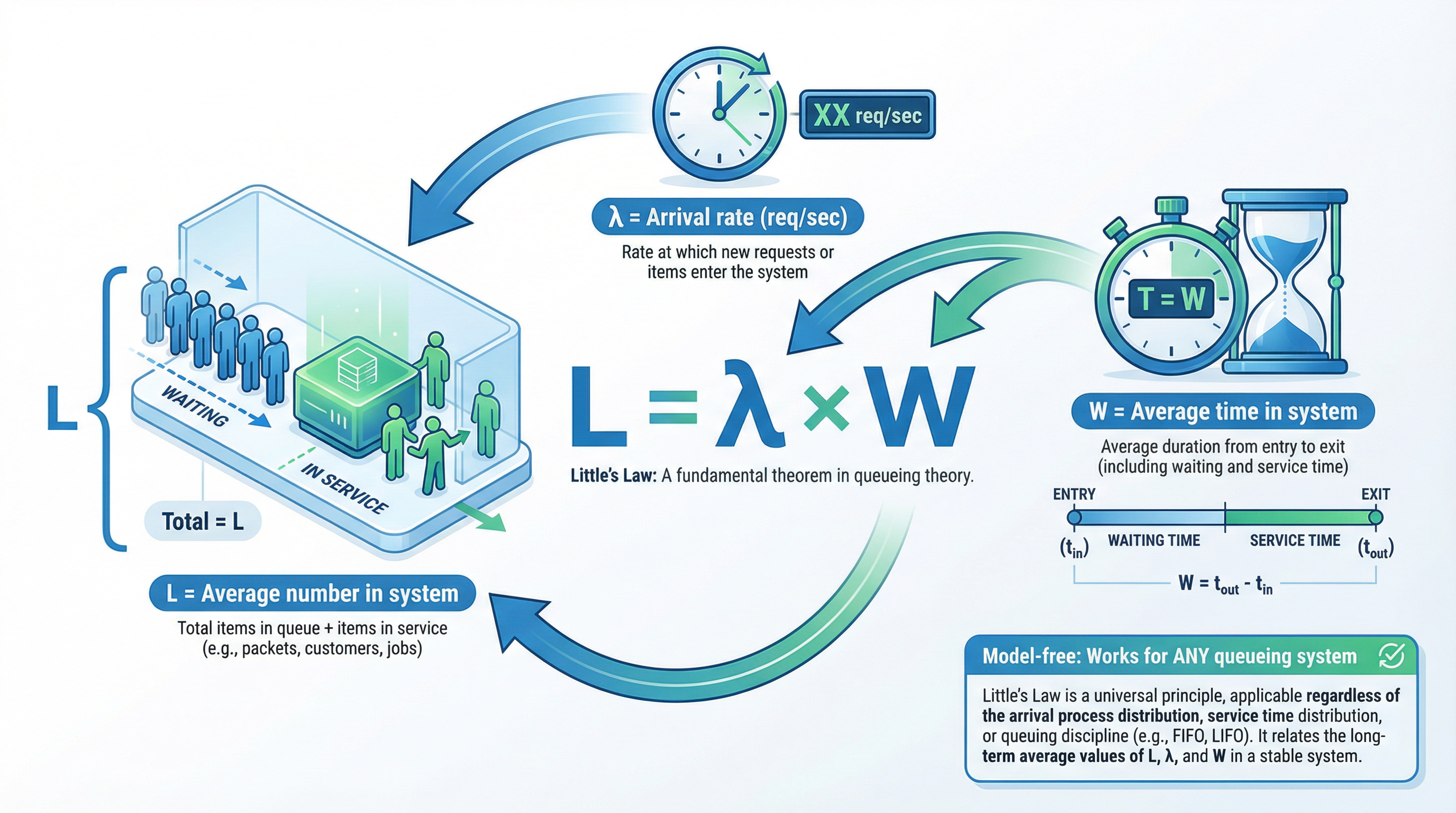
Example: If your system handles 200 req/s and the average request spends 0.25s end-to-end, then \(L = 200 \times 0.25 = 50\) requests in-flight.

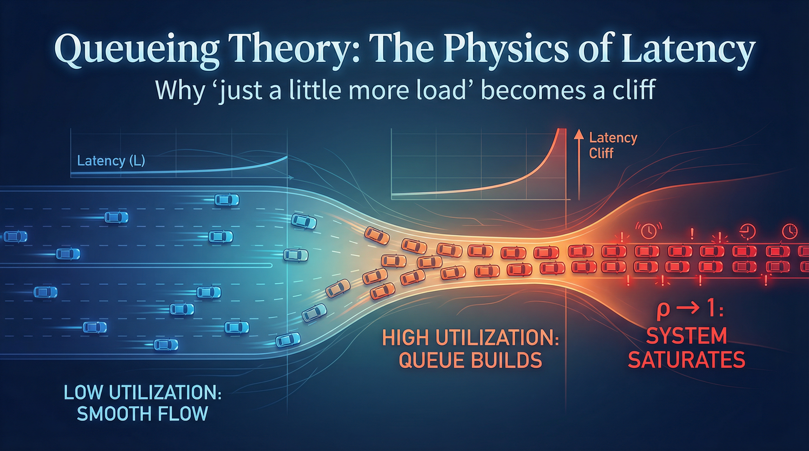
25.3 The Latency Cliff

For an M/M/1 queue (Poisson arrivals, exponential service time), the expected latency is: [2]

\[W = \frac{1}{\mu - \lambda}\]

This equation shows the latency cliff: as \(\lambda \to \mu\), latency diverges.

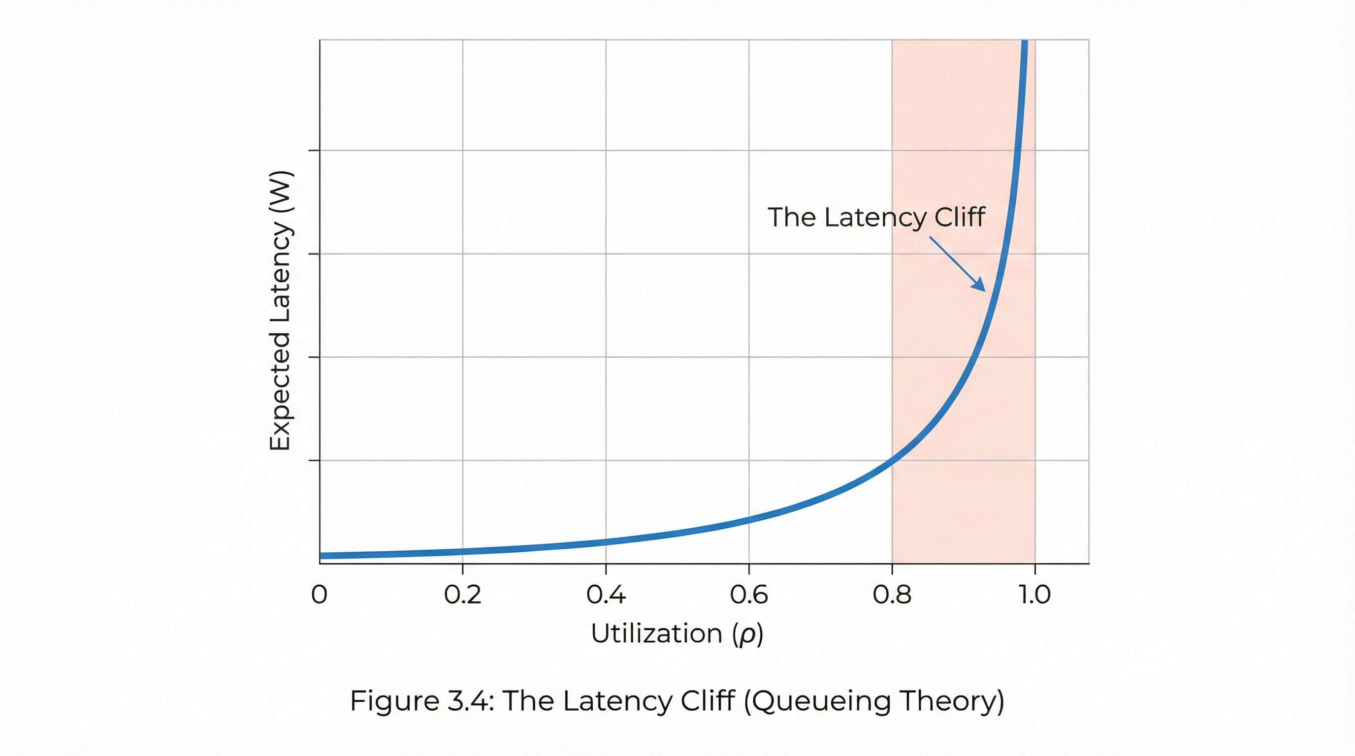
Utilization (ρ)   Expected W (in units of mean service time)
0.50              2×
0.80              5×
0.90              10×
0.95              20×

If your average service time is 50 ms, then 90% utilization implies ~500 ms mean latency. The tail is worse.

Takeaway: High utilization is the enemy of tail latency.

NoteInteractive: Utilization vs Latency

Move utilization toward 1 and watch latency explode.

viewof utilization = Inputs.range([0.05, 0.98], {
  value: 0.8,
  step: 0.01,
  label: "Utilization (ρ)"
})

viewof meanServiceMs = Inputs.range([5, 200], {
  value: 50,
  step: 5,
  label: "Mean service time (ms)"
})

meanServiceSec = meanServiceMs / 1000
expectedW = meanServiceSec / (1 - utilization)
queueDelay = expectedW - meanServiceSec
slowdown = expectedW / meanServiceSec

html`
<div style="font-family: monospace; padding: 1rem; background: #f5f5f5; border-radius: 8px;">
  <div><strong>Mean service time:</strong> ${meanServiceMs.toFixed(0)} ms</div>
  <div><strong>Expected mean latency (W):</strong> ${(expectedW * 1000).toFixed(1)} ms</div>
  <div><strong>Queueing delay (Wq):</strong> ${(queueDelay * 1000).toFixed(1)} ms</div>
  <div><strong>Slowdown (W / E[S]):</strong> ${slowdown.toFixed(1)}×</div>
</div>
`

25.4 Variability Drives Tails

Two systems can have the same average service time but wildly different tails.

For M/D/1 (deterministic service time):

\[W_q = \frac{\rho^2}{2\mu(1-\rho)}\]

For M/M/1 (exponential service time):

\[W_q = \frac{\rho}{\mu - \lambda}\]

Same mean, different variance, different queues.

A useful approximation for general systems is Kingman’s formula: [2]

\[W_q \approx \frac{\rho}{1-\rho} \cdot \frac{c_a^2 + c_s^2}{2} \cdot E[S]\]

Where \(c_a\) and \(c_s\) are the coefficients of variation of inter-arrival and service times.

Translation: Variability is multiplicative with utilization. Reduce variance, reduce tail latency.

NoteInteractive: Variability Penalty (Kingman)

Explore how arrival/service variability amplifies queueing delay.

viewof utilK = Inputs.range([0.05, 0.98], {
  value: 0.8,
  step: 0.01,
  label: "Utilization (ρ)"
})

viewof meanServiceMsK = Inputs.range([5, 200], {
  value: 50,
  step: 5,
  label: "Mean service time E[S] (ms)"
})

viewof ca = Inputs.range([0.1, 3], {
  value: 1,
  step: 0.1,
  label: "Arrival variability (c_a)"
})

viewof cs = Inputs.range([0.1, 3], {
  value: 1,
  step: 0.1,
  label: "Service variability (c_s)"
})

meanServiceSecK = meanServiceMsK / 1000
kingmanWq = (utilK / (1 - utilK)) * ((ca ** 2 + cs ** 2) / 2) * meanServiceSecK
kingmanW = kingmanWq + meanServiceSecK

html`
<div style="font-family: monospace; padding: 1rem; background: #f5f5f5; border-radius: 8px;">
  <div><strong>Queueing delay (Wq):</strong> ${(kingmanWq * 1000).toFixed(1)} ms</div>
  <div><strong>Total mean latency (W):</strong> ${(kingmanW * 1000).toFixed(1)} ms</div>
  <div><strong>Variability factor:</strong> ${(((ca ** 2 + cs ** 2) / 2)).toFixed(2)}</div>
</div>
`

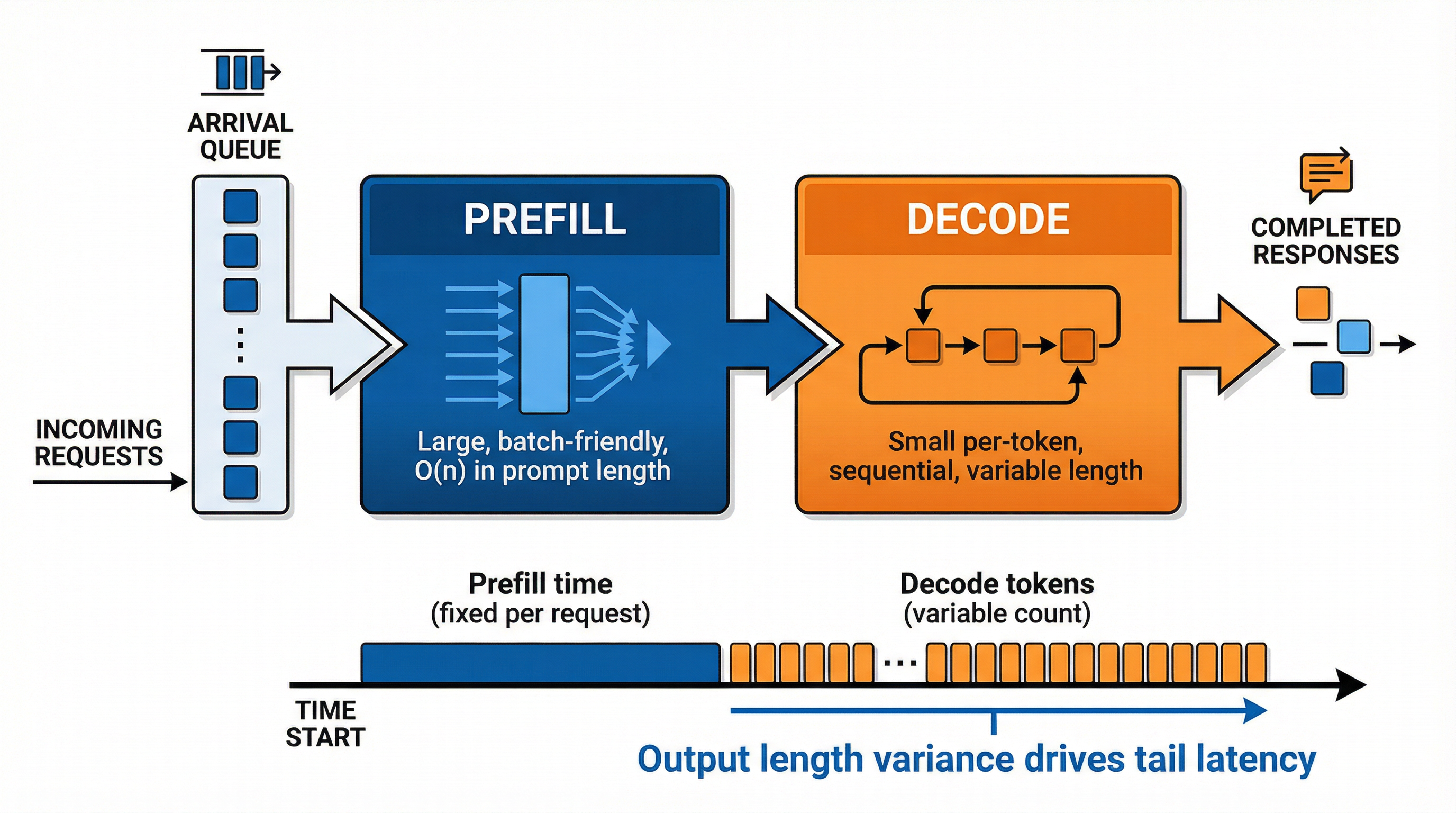
25.5 Two-Phase Service: Prefill + Decode

LLM serving is not a single service time. It is at least two phases:

1. Prefill (prompt processing): large, batch-friendly
2. Decode (token-by-token): small, sequential, highly variable

If a request’s total service time is:

\[S = S_{prefill} + n_{tokens} \cdot S_{decode}\]

then variance comes from output length. Long generations create heavy tails even if the mean is small.

Mitigations:

• Separate queues for prefill and decode
• Predict or cap output length
• Prioritize short requests (Shortest Remaining Processing Time, SRPT)

25.6 Batching: The Throughput Tradeoff

Batching improves throughput but adds batching delay.

If you wait for a batch of size \(b\), the expected waiting time to fill the batch is roughly:

\[W_{batch} \approx \frac{b - 1}{2\lambda} \quad \text{(Poisson arrivals)}\]

Total latency becomes:

\[W \approx W_{queue} + W_{batch} + W_{service}\]

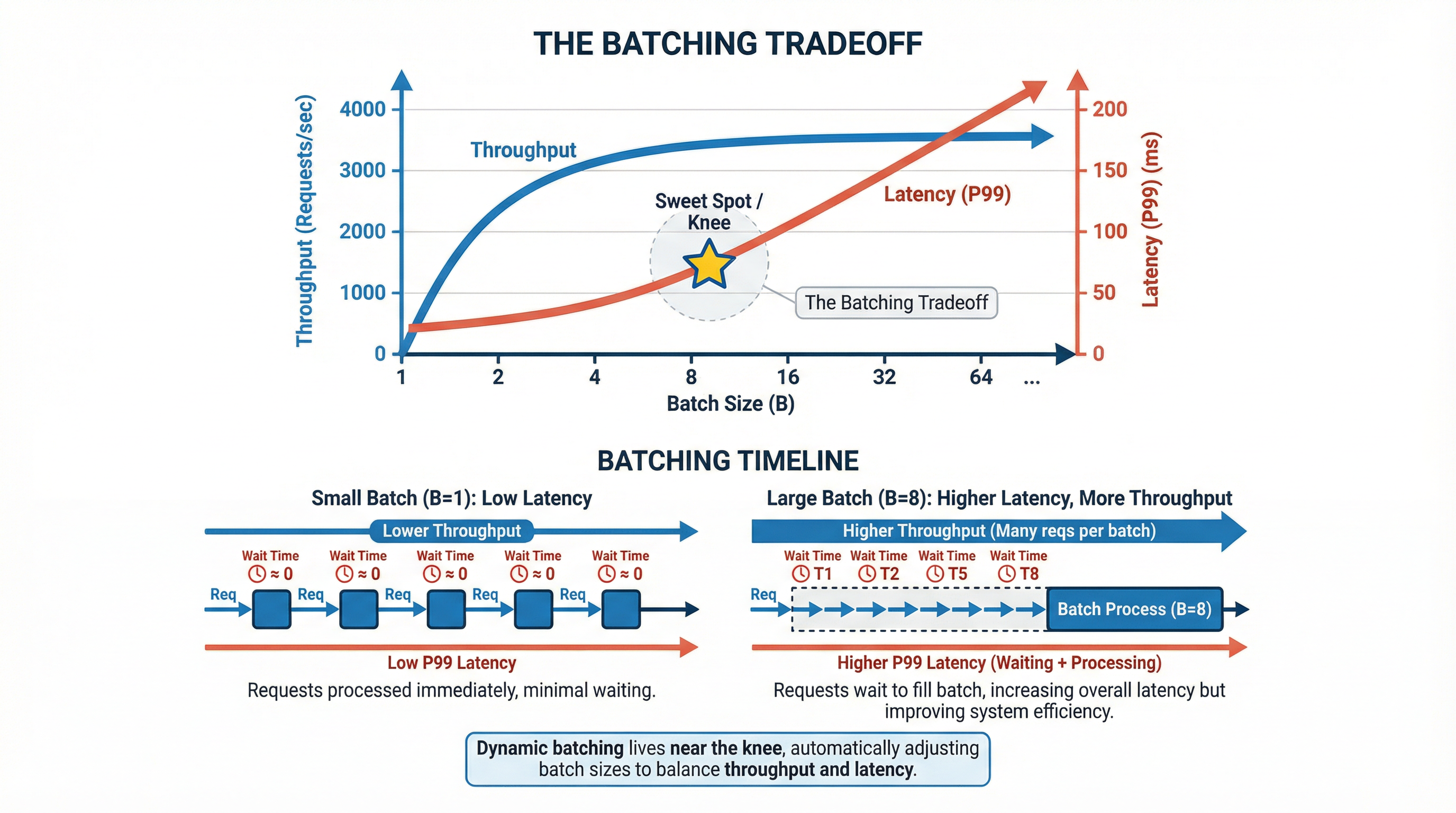
Dynamic batching tries to live near the knee: enough batch size to raise \(\mu\), but not so much delay that P99 explodes.

25.7 Control Levers

When P99 is too high, you have only a few knobs:

• Reduce utilization: add capacity or shed load
• Reduce variance: cap output length, normalize prompt sizes, separate phases
• Improve scheduling: priority queues, preemption, SRPT
• Admission control: token bucket or adaptive concurrency limits to prevent entering unstable regions

Admission control is often the safest lever: reject or defer excess work early so the system never crosses \(\rho \approx 1\).

These are structural levers, not micro-optimizations.

25.8 Measurement Checklist

Track these explicitly:

• Arrival rate \(\lambda\)
• Service time distribution (not just mean)
• Queue length over time
• P50/P95/P99 for queue time and service time separately

If you only measure end-to-end latency, you cannot tell whether the problem is compute or queueing.

25.9 Mini Case Study

Assume:

• Average service time \(E[S] = 0.25s\) (so \(\mu = 4\) req/s)
• Arrival rate \(\lambda = 3.2\) req/s (80% utilization)

Then:

\[W \approx \frac{1}{\mu - \lambda} = \frac{1}{0.8} = 1.25s\]

Your average latency is 5× your mean service time — and P99 will be worse.

This is why systems that “look fine” at 60% utilization fall apart at 80%.

25.10 Connections

• Inference Optimization: Prefill and decode have different queueing behavior. See Inference Optimization.
• The Art of Measurement: Queueing metrics are a first-class signal. See The Art of Measurement.
• Advanced LLM Serving: Admission control, batching, and prioritization are queueing levers. See Advanced LLM Serving.

25.11 Key Takeaways

1. Utilization predicts tail latency: \(\rho \to 1\) implies runaway queues.
2. Variance matters as much as mean: lower service time variance lowers tails.
3. Batching is a tradeoff: throughput up, latency up.
4. Queue time is diagnosable: measure it separately from service time.

[1]

J. D. C. Little, “A proof for the queueing formula: L = \(\lambda\)w,” Operations Research, vol. 9, no. 3, pp. 383–387, 1961.

[2]

M. Harchol-Balter, Performance modeling and design of computer systems: Queueing theory in action. Cambridge University Press, 2013.