29 The Art of Analogy
Finding Related Problems That Have Been Solved
Pólya’s most powerful heuristic: “Do you know a related problem?”
The best performance engineers don’t reinvent solutions. They recognize when a new problem is secretly an old problem in disguise.
This chapter is about building that recognition.
29.2 How Analogies Work
An analogy maps structure from a source domain (well-understood) to a target domain (new problem).
Source: Streaming aggregation (databases)
Target: Attention (deep learning)

Mapping:
  sum(values)           →  softmax weighted sum
  running total         →  running (max, sum, output)
  one-pass constraint   →  memory efficiency
  associativity         →  chunking

Result: FlashAttention
The power comes from structure preservation. If two problems have the same structure, they have the same solution—translated.
29.3 Case Study: From Databases to FlashAttention
Let’s trace an actual analogy.
29.3.1 The Source Problem: Online Aggregation
Databases have computed aggregates for decades:
SELECT AVG(value) FROM big_tableFor a table that doesn’t fit in memory, you need a streaming algorithm:
def streaming_average(stream):
    """Compute average without storing all values"""
    total = 0
    count = 0
    for value in stream:
        total += value
        count += 1
    return total / count
Key insight: We maintain running state and update it incrementally.
29.3.2 The Target Problem: Attention
Standard attention:
def attention(Q, K, V):
    scores = Q @ K.T / sqrt(d)
    weights = softmax(scores)  # Requires all scores at once
    output = weights @ V
    return output
Softmax seems to require all values simultaneously:
def softmax(x):
    exp_x = exp(x - max(x))  # Need max of all values
    return exp_x / sum(exp_x)  # Need sum of all values
This is analogous to:
def normalized_sum(values, weights):
    weighted = [w * v for w, v in zip(weights, values)]
    return sum(weighted) / sum(weights)
Both need to see all values to normalize. Or do they?
29.3.3 The Analogy
Database insight: Many “need all values” operations have streaming equivalents via associativity.
# Running average
def streaming_avg(stream):
    total = 0
    count = 0
    for value in stream:
        total += value
        count += 1
    return total / count  # Normalize at the end
Can we do the same for softmax? The max-stable trick:
def streaming_softmax_sum(stream):
    """Compute sum(exp(x_i - max)) and max in one pass"""
    running_max = float('-inf')
    running_sum = 0

    for value in stream:
        if value > running_max:
            # Rescale previous sum
            running_sum = running_sum * exp(running_max - value)
            running_max = value
        running_sum += exp(value - running_max)

    return running_max, running_sum
The weighted output uses the same trick:
def streaming_weighted_sum(stream):
    """Compute softmax-weighted sum in one pass"""
    running_max = float('-inf')
    running_sum = 0
    running_output = 0

    for score, value in stream:
        if score > running_max:
            scale = exp(running_max - score)
            running_sum *= scale
            running_output *= scale
            running_max = score
        weight = exp(score - running_max)
        running_sum += weight
        running_output += weight * value

    return running_output / running_sum
This is the core of FlashAttention. The analogy:
Database streaming     →  Attention streaming
─────────────────────────────────────────────
running total          →  running (max, sum, output)
update per item        →  update per K-V block
normalize at end       →  divide by running sum
29.3.4 The Transfer
Once you recognize the analogy, the solution structure transfers:
- Chunking (from streaming): Process in blocks that fit in memory
- Running state (from aggregation): Maintain (max, sum, output) tuple
- Rescaling (from numerical stability): Use max-stable exponentials
The database community solved this decades ago. FlashAttention rediscovered it.
29.4 Case Study: Momentum as Biased Search
Another powerful analogy connects optimization dynamics to biased search. The payoff is performance: fewer iterations to reach the same quality.
29.4.1 The Source Problem: Biased Binary Search
Classic binary search splits the interval in half because it assumes the target is uniformly distributed. If you have a prior (the target is likely closer to one side), you can split asymmetrically:
mid = left + p * (right - left) # p != 0.5Pick p to match your belief. This is just an asymmetric split based on a prior (not interpolation search). When the bias is right, expected search time drops.
29.4.2 The Target Problem: Gradient Descent with Momentum
Plain gradient descent steps in the direction of the current gradient:
\[x_{t+1} = x_t - \eta g_t\]
where \(g_t = \nabla f(x_t)\).
Momentum adds inertia. It assumes the next gradient will look like the last:
\[v_{t+1} = \beta v_t + g_t\] \[x_{t+1} = x_t - \eta v_{t+1}\]
Nesterov momentum uses a look-ahead correction:
\[v_{t+1} = \beta v_t + g(x_t - \eta \beta v_t)\] \[x_{t+1} = x_t - \eta v_{t+1}\]
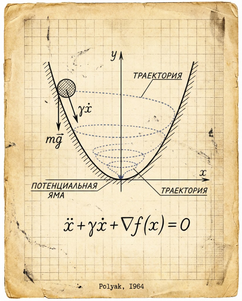
Intuition: in narrow valleys, plain GD zig-zags; momentum smooths the path by carrying direction across steps.

The original momentum analogy is a damped ball rolling in a potential well. Labels are in Russian, but the geometry is the point.
29.4.3 The Analogy
Biased binary search        →  Momentum descent
────────────────────────────────────────────────
Prior over target location  →  Prior over gradient direction
Asymmetric split            →  Inertial (biased) step
Wrong bias costs extra      →  Oscillation / overshoot
In both cases, you spend more effort in the direction you believe is right. If the structure holds (smooth objective, correlated gradients), you get faster convergence. If not, you pay for the bias.
29.4.4 The Transfer
The structural lesson is not “always use momentum.” It’s:
- Exploit temporal coherence: If gradients are correlated, reuse direction.
- Bias cautiously: Larger \(\beta\) is a stronger prior, not a free lunch.
- Measure in iterations: Performance is steps × cost/step.
29.4.5 When the Analogy Breaks
Biased search fails when the prior is wrong. Momentum fails when:
- Gradients are noisy or non-stationary
- Curvature changes sharply (narrow valleys, sharp minima)
- The loss surface has frequent direction reversals
The fix is the same: weaken the bias (smaller \(\beta\), adaptive schedules).
Recent optimizers (for example, Muon) revisit the same idea: treat momentum as a bias toward persistent direction, then tune how strongly you trust it under noise and curvature. The details evolve quickly; the structural question stays the same: does the bias improve progress per step for your objective?
29.5 The Pattern Library
Over time, you build a library of patterns that keep recurring. Here are the most useful:
29.5.1 Pattern: Divide and Conquer
Source: Mergesort, quicksort, binary search
Structure: Split problem in half, solve recursively, combine results.
Transfers to: - Cache-oblivious algorithms (recursive tiling) - Parallel reduction (split work among threads) - Hierarchical attention (split sequence, combine)
# The universal pattern
def divide_conquer(problem):
    if is_base_case(problem):
        return solve_directly(problem)
    left, right = split(problem)
    left_result = divide_conquer(left)
    right_result = divide_conquer(right)
    return combine(left_result, right_result)
29.5.2 Pattern: Lazy Evaluation
Source: Functional programming, demand paging
Structure: Don’t compute until needed. Cache results.
Transfers to: - JIT compilation (compile only executed paths) - Lazy tensor materialization (don’t allocate until used) - Copy-on-write (share until modification)
# The universal pattern
class Lazy:
    def __init__(self, computation):
        self.computation = computation
        self.cached = None

    def get(self):
        if self.cached is None:
            self.cached = self.computation()
        return self.cached
29.5.3 Pattern: Amortization
Source: Dynamic arrays, splay trees
Structure: Occasional expensive operations average out to cheap.
Transfers to: - Gradient checkpointing (trade recompute for memory) - Memory pools (occasional allocation, fast reuse) - Batched operations (overhead per batch, not per item)
# The universal pattern: occasional O(n), amortized O(1)
class DynamicArray:
    def append(self, item):
        if len(self.data) == self.capacity:
            self.resize(2 * self.capacity)  # Rare O(n)
        self.data.append(item)  # Common O(1)
29.5.4 Pattern: Memoization
Source: Dynamic programming, caching
Structure: Don’t recompute what you’ve computed before.
Transfers to: - KV cache in transformers (don’t recompute past attention) - Compiled kernel caching (don’t recompile same shapes) - Feature caching (store intermediate activations)
# The universal pattern
cache = {}
def memoized(f):
    def wrapper(*args):
        if args not in cache:
            cache[args] = f(*args)
        return cache[args]
    return wrapper
29.5.5 Pattern: Trading Space for Time
Source: Hash tables, lookup tables
Structure: Precompute and store to avoid runtime computation.
Transfers to: - Lookup tables for activation functions - Storing attention weights vs. recomputing - Materialized views vs. queries
29.5.6 Pattern: Trading Time for Space
Source: Compression, streaming
Structure: Recompute instead of storing.
Transfers to: - Gradient checkpointing - Streaming algorithms - Recomputing activations instead of caching
29.5.7 Pattern: Approximation
Source: Monte Carlo, compressed sensing
Structure: Trade exactness for efficiency.
Transfers to: - Stochastic gradient descent (approximate full gradient) - Quantization (approximate full precision) - Sparse attention (approximate full attention)
29.6 Cross-Domain Transfer
The most powerful analogies come from outside your domain.
29.6.1 From Physics: Conservation Laws
In physics, many systems satisfy conservation laws:
Energy in = Energy out + Energy storedIn computing, we have analogous constraints:
Data in = Data out + Data buffered
Work = Compute × Time = Bandwidth × Data
This leads to insights like:
- Little’s Law: Throughput = Parallelism / Latency
- Amdahl’s Law: Speedup = 1 / (Serial + Parallel/P)
- Bandwidth-bound: Time ≥ Data / Bandwidth
29.6.2 From Economics: Supply and Demand
Economic thinking transfers surprisingly well:
Economics                    Computing
─────────────────────────────────────────
Scarce resource              Memory/compute
Market equilibrium           Load balancing
Arbitrage                    Optimization opportunity
Diminishing returns          Amdahl's law
Opportunity cost             Time vs. space tradeoff
When optimizing a system, ask: - What’s the scarce resource? - Where’s the “arbitrage opportunity” (unused capacity)? - What’s the opportunity cost of this approach?
29.6.3 From Biology: Evolution
Evolution has solved optimization problems for billions of years:
Mutation         →  Random search, perturbation
Selection        →  Gradient descent, keeping improvements
Adaptation       →  Auto-tuning, learning schedules
Niches           →  Specialized hardware, accelerators
Many ML optimization techniques are literally inspired by evolution.
29.6.4 From Civil Engineering: Capacity Planning
Traffic engineers study flow and congestion:
Traffic                      Computing
─────────────────────────────────────────
Road capacity                Bandwidth
Vehicles                     Data/requests
Congestion                   Queueing
Rush hour                    Peak load
Alternative routes           Load balancing
Bottleneck (single lane)     Amdahl's serial portion
Queueing theory from traffic engineering is fundamental to systems performance.
29.7 When Analogies Fail
Analogies are powerful but dangerous. They can mislead.
29.7.1 Failure Mode: Surface Similarity
"Attention is like a database query"
  Similarity: Both find relevant items
  Difference: Attention uses soft weighting, not filtering

"Neural networks are like brains"
  Similarity: Both compute
  Difference: Almost everything else

Danger: Optimizations that work for one may not work for the other
29.7.2 Failure Mode: Wrong Abstraction Level
"GPU is like CPU but faster"
  Similarity: Both execute instructions
  Difference: Completely different architecture

Danger: CPU optimizations (branch prediction, OoO execution)
don't transfer to GPU29.7.4 How to Know When Analogies Fail
Test the mapping explicitly:
1. List the key properties of the source solution
2. Map each property to the target domain
3. Check if each mapped property holds
4. If any fail, the analogy may break there
Example:
Source: Merge sort parallelization
Property: Work can be divided evenly
Target: Training neural networks

Mapping: Can we divide training work evenly?
Check: Yes, data parallel splits batches evenly ✓

Mapping: Is combine step cheap?
Check: Gradient averaging is cheap ✓

Mapping: Are subproblems independent?
Check: Mostly, except for batch normalization ✗

Conclusion: Analogy mostly works, but breaks for batch norm
29.8 Building Your Pattern Library
29.8.1 Step 1: Study Classic Algorithms
The classics are classics for a reason:
Required reading:
- CLRS (algorithms)
- Hennessy & Patterson (computer architecture)
- Silberschatz (operating systems)
- Gray & Reuter (database systems)

Each contains dozens of transferable patterns.
29.8.2 Step 2: Understand the Why, Not Just the What
Learning mergesort:
  What: Divide, sort halves, merge
  Why:  Exploits divide-and-conquer for O(n log n)
        Merge is O(n) because inputs are sorted

The "why" transfers. The "what" is just one instantiation.
29.8.3 Step 3: Practice Pattern Recognition
When you see a solution:
- What pattern is it using?
- What are the key structural properties?
- Where else could this pattern apply?
FlashAttention: "That's streaming aggregation!"
LoRA: "That's low-rank matrix factorization!"
MoE: "That's adaptive compute allocation!"
29.8.4 Step 4: Cross-Pollinate
Read outside your field:
- Databases → Memory management patterns
- Compilers → Optimization passes
- Graphics → GPU programming patterns
- Networking → Distributed systems patterns
- Biology → Optimization algorithms
The best insights come from unexpected connections.
29.9 The Meta-Pattern
All the patterns we’ve seen share a structure:
1. Identify the constraint (memory, compute, bandwidth, latency)
2. Find a property that enables working around it
   (associativity, separability, locality, approximability)
3. Design an algorithm that exploits that property on hardware
4. Implement with attention to hardware details
This is the meta-pattern of performance engineering:
Properties enable algorithms. Hardware constrains implementations. The art is connecting them.
29.10 Key Takeaways
Related problems accelerate solutions: Don’t reinvent. Recognize and adapt.
Build a pattern library: Divide-and-conquer, memoization, lazy evaluation, amortization—these recur everywhere.
Cross-domain analogies are powerful: Databases, physics, economics, biology—all have transferable insights.
Test analogies carefully: Surface similarity can mislead. Check that structural properties actually transfer.
Understand the “why”: The mechanism transfers, not the implementation.
The best performance engineers are collectors of patterns. Every new problem is an opportunity to recognize an old friend in new clothes.
The accompanying notebook lets you:
- Practice pattern recognition on sample problems
- Build your own pattern library
- Test analogies with explicit property mapping
- Explore cross-domain transfers
![]()
29.11 Further Reading
- Pólya (1945). “How to Solve It” (especially Chapter 2: How to Solve It)
- Hofstadter (2001). “Analogy as the Core of Cognition”
- Gentner (1983). “Structure-Mapping: A Theoretical Framework for Analogy”
- McConnell (2004). “Code Complete” (Chapter 2: Metaphors for a Richer Understanding)
29.12 Conclusion: The Nature of Fast
We’ve reached the end of our investigation.
We started with a question: Why are some programs fast and others slow?
The answer is not magic. It’s not about knowing secret tricks. It’s about understanding properties—mathematical properties that enable algorithmic optimization, and hardware properties that reward certain access patterns.
Associativity enables chunking and parallelism. Separability enables factorization and low-rank approximation. Sparsity enables conditional computation. Locality enables cache efficiency.
These properties don’t exist in isolation. They compose. FlashAttention uses associativity and locality. LoRA uses separability and sparsity. The best algorithms use all of them.
Hardware doesn’t care about your algorithm’s elegance. It cares about: - Memory access patterns - Arithmetic intensity - Parallelism without synchronization - Data that stays close to compute
The art of performance engineering is matching algorithmic properties to hardware constraints. Find the properties your problem has. Exploit them on real hardware. Measure. Iterate.
This is the nature of fast.